Setting-Up an MPC Controller

Table of Contents

• Mathematical Formulation of Model Predictive Control Problems
• Implementation of an MPC Controller for a Quarter Car
• List of RealTimeAlgorithm Options

This tutorial explains how to setup a basic MPC controller. Again, we consider a simple actively damped quarter car model.

Mathematical Formulation of Model Predictive Control Problems

Let x denote the states, u the control input, p a time-constant parameter, and T the time horizon of an MPC optimization problem. We are interested in tracking MPC problems, which are of the general form:

Here, the function f represents the model equations, s the path constraints and r the terminal constraints. Note that in the online context, the above problem must be solved iteratively for changing x0 and t0 . Moreover, we assume here that the objective is given in least square form. Most of the tracking problems that arise in practice can be formulated in this form with η and μ denoting the tracking and terminal reference.

Implementation of an MPC Controller for a Quarter Car

The following piece of code shows how to implement an MPC controller based on this quarter car model. It comprises six main steps:

1. Introducing all variables and constants.
2. Setting up the quarter car ODE model.
3. Setting up a least-squares objective function by defining the five components of the measurement function h and an appropriate weighting matrix.
4. Defining a complete optimal control problem (OCP) comprising the dynamic model, the objective function as well as constraints on the input.
5. Setting up a RealTimeAlgorithm defined by the OCP to be solved at each sampling instant together with a sampling time specifying the time lag between two sampling instants. Moreover, several options can be set and plot windows flushed.
6. Setting up a Controller by specifying a control law, i.e. the real-time algorithm solving our OCP in this case, and a reference trajectory to be tracked. In this example, the reference trajectory is read from a file where the value of all components are defined over time. (Note that the reference trajectory can be left away when calling the Controller constructor which is equivalent to all entries zero over the whole simulation horizon.)

#include <acado_toolkit.hpp>
#include <include/acado_gnuplot/gnuplot_window.hpp>

int main( )
{
    USING_NAMESPACE_ACADO


    // INTRODUCE THE VARIABLES:
    // -------------------------
    DifferentialState xB;
    DifferentialState xW;
    DifferentialState vB;
    DifferentialState vW;

    Control F;
    Disturbance R;

    double mB = 350.0;
    double mW = 50.0;
    double kS = 20000.0;
    double kT = 200000.0;


    // DEFINE A DIFFERENTIAL EQUATION:
    // -------------------------------
    DifferentialEquation f;

    f << dot(xB) == vB;
    f << dot(xW) == vW;
    f << dot(vB) == ( -kS*xB + kS*xW + F ) / mB;
    f << dot(vW) == ( -kT*xB - (kT+kS)*xW + kT*R - F ) / mW;


    // DEFINE LEAST SQUARE FUNCTION:
    // -----------------------------
    Function h;

    h << xB;
    h << xW;
    h << vB;
    h << vW;
    h << F;

    // LSQ coefficient matrix
    Matrix Q(5,5);
    Q(0,0) = 10.0;
    Q(1,1) = 10.0;
    Q(2,2) = 1.0;
    Q(3,3) = 1.0;
    Q(4,4) = 1.0e-8;

    // Reference
    Vector r(5); 
    r.setAll( 0.0 );


    // DEFINE AN OPTIMAL CONTROL PROBLEM:
    // ----------------------------------
    const double tStart = 0.0;
    const double tEnd   = 1.0;

    OCP ocp( tStart, tEnd, 20 );

    ocp.minimizeLSQ( Q, h, r );

    ocp.subjectTo( f );

    ocp.subjectTo( -200.0 <= F <= 200.0 );
    ocp.subjectTo( R == 0.0 );


    // SETTING UP THE REAL-TIME ALGORITHM:
    // -----------------------------------
    RealTimeAlgorithm alg( ocp,0.025 );
    alg.set( MAX_NUM_ITERATIONS, 1 );
    alg.set( PLOT_RESOLUTION, MEDIUM );

    GnuplotWindow window;
                window.addSubplot( xB, "Body Position [m]" );
                window.addSubplot( xW, "Wheel Position [m]" );
                window.addSubplot( vB, "Body Velocity [m/s]" );
                window.addSubplot( vW, "Wheel Velocity [m/s]" );
                window.addSubplot( F,  "Damping Force [N]" );
                window.addSubplot( R,  "Road Excitation [m]" );

    alg << window;


    // SETUP CONTROLLER AND PERFORM A STEP:
    // ------------------------------------
    StaticReferenceTrajectory zeroReference( "ref.txt" );

    Controller controller( alg,zeroReference );

    Vector y( 4 );
    y.setZero( );
    y(0) = 0.01;

    controller.init( 0.0,y );
    controller.step( 0.0,y );


    return 0;
}

The file "ref.txt" contains the data of the (trivial) reference trajectory:

DATA FILE: ref.txt

--------------------------------------------

TIME    xB      xW      vB      vW      F

0.0     0.00    0.00    0.00    0.00    0.00
1.0     0.00    0.00    0.00    0.00    0.00
1.5     0.00    0.00    0.00    0.00    0.00
2.0     0.00    0.00    0.00    0.00    0.00
3.0     0.00    0.00    0.00    0.00    0.00

--------------------------------------------

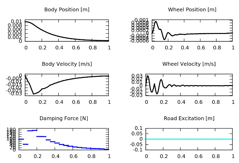
If we run the above piece of code in ACADO, the corresponding Gnuplot output should be as follows:

Simulation results

List of RealTimeAlgorithm Options

We end this tutorial with providing lists comprising the most common options that can be set when defining a RealTimeAlgorithm:

Option Name:	Option Value:	Short Description:
MAX_NUM_ITERATIONS	int	maximum number of SQP iterations (by default, only one SQP iteration is performed)
USE_REALTIME_ITERATIONS	YES NO	specifying whether real-time iterations shall be used or not
USE_IMMEDIATE_FEEDBACK	YES NO	specifying whether immediate feedback shall be given or not
KKT_TOLERANCE	double	termination tolerance for the optimal control algorithm
HESSIAN_APPROXIMATION	CONSTANT_HESSIAN FULL_BFGS_UPDATE BLOCK_BFGS_UPDATE GAUSS_NEWTON EXACT_HESSIAN	constant hessian (generalized gradient method) BFGS update of the whole hessian structure-exploiting BFGS update (default) Gauss-Newton Hessian approximation (only for LSQ) exact Hessian computation
DISCRETIZATION_TYPE	SINGLE_SHOOTING MULTIPLE_SHOOTING COLLOCATION	single shooting discretization multiple shooting discretization (default) collocation (will be implemented soon)
INTEGRATOR_TYPE	INT_RK12 INT_RK23 INT_RK45 INT_RK78 INT_BDF	Runge Kutta integrator (adaptive Euler method) Runge Kutta integrator (order 2/3, RKF ) Runge Kutta integrator (order 4/5, Dormand Prince) Runge Kutta integrator (order 7/8, Dormand Prince) BDF (backward differentiation formula) integrator
INTEGRATOR_TOLERANCE	double	the relative tolerance of the integrator
ABSOLUTE_TOLERANCE	double	the absolute tolerance of the integrator ("ATOL")
LEVENBERG_MARQUARDT	double	value for Levenberg-Marquardt regularization
PLOT_RESOLUTION	LOW MEDIUM HIGH	specifying screen resolution when plotting

Next example: Setting-Up More Classical Feedback Controllers