This tutorial explains how to set up multi-objective optimal control problems in ACADO. As an example the optimal and safe operation of a jacketed tubular reactor is considered. Inside the tubular reactor an exothermic irreversible first order reaction takes place. The heat produced by this reaction is removed through the surrounding jacket. In addition, it is assumed that the reactor operates in steady-state conditions and that the fluid flow as a plug through the tube. The aim is to find an optimal profile along the reactor for the temperature of the fluid in the jacket such that conversion and energy costs are minimized.
Mathematical formulation
The optimal control problem involves two states: the dimensionless temperature x1 and the dimensionless reactant concentration x2 and one control: the dimensionless jacket fluid temperature u . The reactor length has been fixed to L. The conversion objective involves the minimization of the reactant concentration at the outlet: CF* (1- x1(L) ) with CF the reactant concentration in the feed stream. The energy objective relates to the minimization of the terminal heat loss by penalizing deviations between the reactor in- and outlet temperature: TF2 / K1 * x22(L) . The conditions at the reactor inlet are given and equal to the values of the feed stream. The dimensionless concentration is intrinsically bounded between 0 and 1, whereas upper and lower constraints are imposed on the jacket and reactor temperatures for safety and constructive reasons.
![\begin{eqnarray*} \begin{array}{lcl} \min_{x(\cdot),u(\cdot)}& & \left\{C_{F}(1-x_1(L)),\frac{T_{F}^2}{K_1}x_2^2(L)\right\} \\ \textrm{subject to:} & & \qquad \quad \quad \\ \forall z \in [0,L]: & & \frac{dx_{1}}{dz} = \frac{\alpha}{v} (1 - x_{1})e^{\frac{\gamma x_{2}}{1+x_{2}}} \\ & & \frac{dx_{2}}{dz} = \frac{\alpha \delta}{v}(1-x_{1})e^{\frac{\gamma x_{2}}{1+x_{2}}} + \frac{\beta}{v} (u - x_{2}) \\ \forall z \in [0,L]: & & 0.0 \leq x_1 \leq 1.0 \\ & & x_{2,\mathrm{min}} \leq x_2 \leq x_{2,\mathrm{max}} \\ & & u_{\mathrm{min}} \leq u \leq u_{\mathrm{max}} \\ \mathrm{at~} z = 0: & & x_{1}(0) = 0.0 \\ & & x_{2}(0) = 0.0 \\ \end{array} \end{eqnarray*}](form_60.png)
Note that the time t as independent variable has been replaced by the spatial coordinate z , since optimal spatial profiles along the length of the reactor are required.
An ACADO tutorial code
The following piece of code illustrates how to set up the multi-objective optimal control problem mentioned above. NBI is used to approximate the Pareto set with 11 points. The pareto front is plotted and exported. Also all corresponding optimal state and control profiles are exported. This code is available in the examples/multi_objective directory as plug_flow_reactor_nbi.cpp. The WS and NNC version are called plug_flow_reactor_ws.cpp and plug_flow_reactor_nnc.cpp, respectively.
#include <acado_optimal_control.hpp>
#include <include/acado_gnuplot/gnuplot_window.hpp>

int main( )
{
    USING_NAMESPACE_ACADO

    // INTRODUCE FIXED PARAMETERS:
    // ---------------------------
    #define  v          0.1
    #define  L          1.0
    #define  Beta       0.2
    #define  Delta      0.25
    #define  E          11250.0
    #define  k0         1E+06
    #define  R          1.986
    #define  K1         250000.0
    #define  Cin        0.02
    #define  Tin        340.0


    // INTRODUCE THE VARIABLES:
    // -------------------------
    DifferentialState     x1,x2;
    Control               u    ;
    DifferentialEquation  f( 0.0, L );


    // DEFINE A DIFFERENTIAL EQUATION:
    // -------------------------------
    double Alpha, Gamma;
    Alpha = k0*exp(-E/(R*Tin));
    Gamma = E/(R*Tin);

    f << dot(x1) ==  Alpha       /v * (1.0-x1) * exp((Gamma*x2)/(1.0+x2));
    f << dot(x2) == (Alpha*Delta)/v * (1.0-x1) * exp((Gamma*x2)/(1.0+x2))
                                               + Beta/v * (u-x2);


    // DEFINE AN OPTIMAL CONTROL PROBLEM:
    // ----------------------------------
    OCP ocp( 0.0, L, 50 );
    // Solve conversion optimal problem
    ocp.minimizeMayerTerm( 0, Cin*(1.0-x1) );
    // Solve energy optimal problem (perturbed by small conversion cost;
    // otherwise the problem is ill-defined.)
    ocp.minimizeMayerTerm( 1, (pow((Tin*x2),2.0)/K1) + 0.005*Cin*(1.0-x1) );

    ocp.subjectTo( f );

    ocp.subjectTo( AT_START, x1 ==  0.0 );
    ocp.subjectTo( AT_START, x2 ==  0.0 );

    ocp.subjectTo(  0.0            <= x1 <=  1.0             );
    ocp.subjectTo( (280.0-Tin)/Tin <= x2 <= (400.0-Tin)/Tin  );
    ocp.subjectTo( (280.0-Tin)/Tin <= u  <= (400.0-Tin)/Tin  );


    // DEFINE A MULTI-OBJECTIVE ALGORITHM AND SOLVE THE OCP:
    // -----------------------------------------------------
    MultiObjectiveAlgorithm algorithm(ocp);

    algorithm.set(INTEGRATOR_TYPE,INT_BDF);
    algorithm.set(KKT_TOLERANCE,1e-9);

    algorithm.set(PARETO_FRONT_GENERATION,PFG_NORMAL_BOUNDARY_INTERSECTION);
    algorithm.set(PARETO_FRONT_DISCRETIZATION,11);

    // Minimize individual objective function
    algorithm.solveSingleObjective(0);

    // Minimize individual objective function
    algorithm.solveSingleObjective(1);

    // Generate Pareto set
    algorithm.solve();

    algorithm.getWeights("plug_flow_reactor_nbi_weights.txt");
    algorithm.getAllDifferentialStates("plug_flow_reactor_nbi_states.txt");
    algorithm.getAllControls("plug_flow_reactor_nbi_controls.txt");


    // VISUALIZE THE RESULTS IN A GNUPLOT WINDOW:
    // ------------------------------------------
    VariablesGrid paretoFront;
    algorithm.getParetoFront( paretoFront );

    GnuplotWindow window1;
      window1.addSubplot( paretoFront,"Pareto Front (conversion vs. energy)",
                                      "OUTLET CONCENTRATION","ENERGY",
                                      PM_POINTS );
    window1.plot( );


    // PRINT INFORMATION ABOUT THE ALGORITHM:
    // --------------------------------------
    algorithm.printInfo();


    // SAVE INFORMATION:
    // -----------------
    FILE *file = fopen("plug_flow_reactor_nbi_pareto.txt","w");
    paretoFront.print();
    file << paretoFront;
    fclose(file);

    return 0;
}
Remarks:
- Exporting the scalarization parameters The sequence of the different values for the scalarization parameters ("weights") can be exported to a .txt file.
algorithm.getWeights("plug_flow_reactor_nbi_weights.txt");
- Exporting the optimal control and state profiles Also the optimal control and state profiles along the Pareto set can be exported as .txt files.
        algorithm.getWeights("plug_flow_reactor_nbi_weights.txt");
        algorithm.getAllDifferentialStates("plug_flow_reactor_nbi_states.txt");
        algorithm.getAllControls("plug_flow_reactor_nbi_controls.txt");
To indicate the order of the different solutions, each time "MOx" is added to the name, with x the position in the series of parametric single objective optimization problems. As in the current case 11 Pareto points are required, the state profiles are named from "MO0plug_flow_reactor_nbi_states.txt" to "MO10plug_flow_reactor_nbi_states.txt" and the control profiles are given names from "MO0plug_flow_reactor_nbi_controls.txt" to "MO10plug_flow_reactor_nbi_controls.txt". Note that corresponding values for the scalarization parameters can be found in the weights file "plug_flow_reactor_nbi_weights.txt".
- Perturbation of energy cost In the current case, a fraction of the conversion cost is added to the energy cost as the pure energy optimal case is not uniquely defined. (There are infinitely many profiles with an outlet temperature equal to the inlet temperature.) However, adding this small focus on conversion leads to chemically consistent and gradual results. Moreover, when comparing the current results to results reported in literature, no significant differences are observed.
        // Define energy cost (perturbed by small conversion cost;
        // otherwise the problem is ill-defined.)
        ocp.minimizeMayerTerm( 1,(pow((Tin*x2),2.0)/K1) + 0.005*Cin*(1.0-x1) );
ACADO results
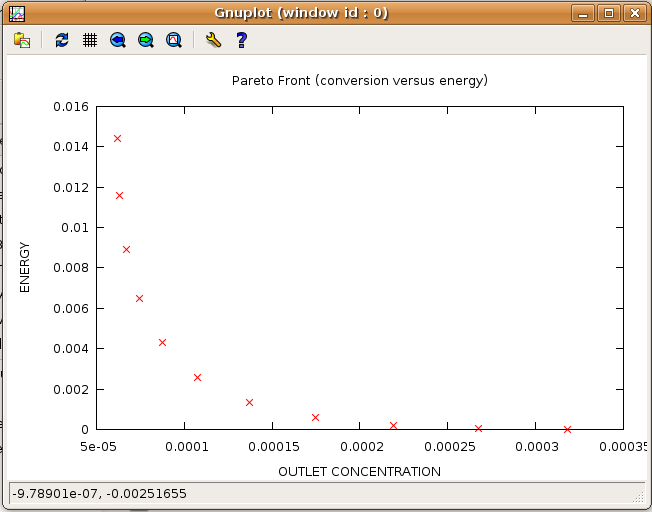
The corresponding Pareto plot as returned by NBI looks as follows in GNUplot:

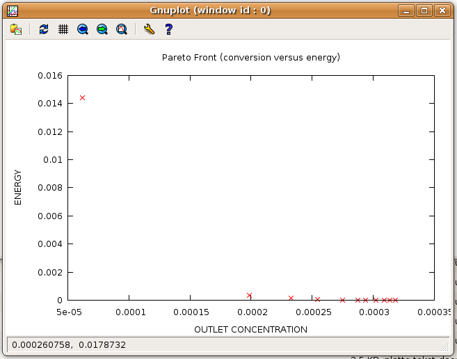
When comparing with the result provided by WS, NBI clearly yields a much nicer spread of the Pareto points along the Pareto front:

Next example: A State and Parameter Estimation Tutorial