A Guiding Example: Time Optimal Control of a Rocket Flight

This tutorial explains how to setup a simple optimal control problem with ACADO. As an example a simple model of a rocket is considered, which should fly as fast as possible from one to another point in space while satisfying state and control constraints during the flight.

Mathematical Formulation of the Optimization Problem:

We consider a simple rocket model with three differential states s, v, and m representing the traveling distance, the velocity, and the mass of the rocket, respectively. Moreover, we assume that the rocket can be accelerated by a control input u . The fuel optimal control problem of our interest has the following form:

Here, the aim is to fly in minimum time T from s(0) = 0 to s(T) = 10 , while constraints on the velocity v and the control input u should be satisfied. Note that the rocket is assumed to start with velocity v(0) = 0 and required to stop at the end time T, which can be formulated in form of the constraint v(T) = 0.

Implementation of the Optimal Control Problem with ACADO Toolkit

The following piece of code shows how to implement the above optimal control problem. In addition, a Gnuplot window is constructed, such that the results can automatically be visualized:

#include <acado_optimal_control.hpp>
#include <include/acado_gnuplot/gnuplot_window.hpp>

int main( )
{
        USING_NAMESPACE_ACADO

        DifferentialState        s,v,m      ;   // the differential states
        Control                  u          ;   // the control input u
        Parameter                T          ;   // the time horizon T
        DifferentialEquation     f( 0.0, T );   // the differential equation

        //-------------------------------------
        OCP ocp( 0.0, T )                   ;   // time horizon of the OCP: [0,T]
        ocp.minimizeMayerTerm( T )          ;   // the time T should be optimized

        f << dot(s) == v                    ;   // an implementation
        f << dot(v) == (u-0.2*v*v)/m        ;   // of the model equations
        f << dot(m) == -0.01*u*u            ;   // for the rocket.

        ocp.subjectTo( f                   );   // minimize T s.t. the model,
        ocp.subjectTo( AT_START, s ==  0.0 );   // the initial values for s,
        ocp.subjectTo( AT_START, v ==  0.0 );   // v,
        ocp.subjectTo( AT_START, m ==  1.0 );   // and m,

        ocp.subjectTo( AT_END  , s == 10.0 );   // the terminal constraints for s
        ocp.subjectTo( AT_END  , v ==  0.0 );   // and v,

        ocp.subjectTo( -0.1 <= v <=  1.7   );   // as well as the bounds on v
        ocp.subjectTo( -1.1 <= u <=  1.1   );   // the control input u,
        ocp.subjectTo(  5.0 <= T <= 15.0   );   // and the time horizon T.
        //-------------------------------------

        GnuplotWindow window                ;   // visualize the results in a
        window.addSubplot( s, "DISTANCE s" );   // Gnuplot window.
        window.addSubplot( v, "VELOCITY v" );
        window.addSubplot( m, "MASS     m" );
        window.addSubplot( u, "CONTROL  u" );

        OptimizationAlgorithm algorithm(ocp);   // construct optimization algorithm,
        algorithm << window                 ;   // flush the plot window,
        algorithm.solve()                   ;   // and solve the problem.

        return 0                            ;
}

This code example is also coming with the ACADO Toolkit and can in this version directly be compiled. The translation of the mathematical formulation into the C++ code should be intuitive. Although, the problem is nonlinear, we do not necessarily need to provide an initialization. Note that the ACADO Toolkit tries to guess an initialization based on the constraints which occur in the problem formulation. Moreover, we did not specify any options regarding the optimization algorithm; the ACADO Toolkit chooses default options. In this example, a multiple shooting discretization with 20 nodes is chosen, while the integration is performed by a Runge-Kutta method (order 4/5). Finally, the optimization of the discretized mathematical program is by default based on a sequential quadratic programming (SQP) method.

A brief discussion of the results

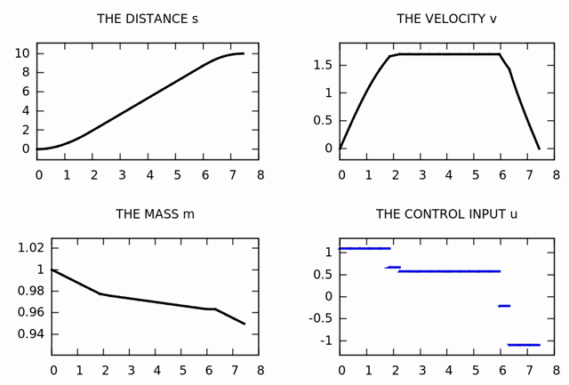
Compiling and running the code should lead to both: An output of the SQP iterations on the terminal as well as a Gnuplot window, which is shown as soon as convergence is achieved. The result shoold look as follows:

Simulation results

The output on the terminal looks as follows:

  1:  KKT tolerance = 4.016e+01    objective value = 9.9500e+00
  2:  KKT tolerance = 1.306e-01    objective value = 9.9316e+00
  3:  KKT tolerance = 2.549e-02    objective value = 9.9061e+00
  4:  KKT tolerance = 7.485e-02    objective value = 9.8314e+00
  5:  KKT tolerance = 3.458e-01    objective value = 9.4875e+00
  6:  KKT tolerance = 3.045e-01    objective value = 9.1909e+00
  7:  KKT tolerance = 5.194e-01    objective value = 8.6915e+00
  8:  KKT tolerance = 4.739e-01    objective value = 8.2481e+00
  9:  KKT tolerance = 3.335e-01    objective value = 7.9276e+00
 10:  KKT tolerance = 4.999e-01    objective value = 7.4579e+00
 11:  KKT tolerance = 1.653e-02    objective value = 7.4419e+00
 12:  KKT tolerance = 1.461e-04    objective value = 7.4417e+00
 13:  KKT tolerance = 1.190e-07    objective value = 7.4417e+00

convergence achieved. 

Here, the optimal results for the three states as well as for the control input are plotted. Note that the time optimal result can quite intuitively be understood: In the first phase, it is optimal to accelerate as fast as possible, i.e. the upper bound constraint for the control input is active. In the second phase, the path constraint for the maximum velocity is active and thus the control input is chosen in such a way that the friction is copensated. Finally, In the third phase, the rocket must brake as fast as possible, i.e. the lower bound constraint is active. Note that in this example only 20 piecewise constant control intervals have been chosen, i.e. the discretiziation of the controls is quite poor in this example.

Next example: Initialization of Nonlinear Optimization Algorithms