Performing a Basic Closed-Loop MPC Simulation

Table of Contents

• Implementation of the MPC Simulation in ACADO

This tutorial explains how to setup a basic closed-loop simulation using a model predictive controller. Again, we consider the simple quarter car model as a guiding example.

Implementation of the MPC Simulation in ACADO

The following piece of code shows how to implement a closed-loop simulation based on our quarter car model. It comprises three main steps:

1. Setting up the ODE model of the quarter car and defining a Process as explained in detail in the online tutorial Setting-Up a Process for MPC Simulations.
2. Setting up an MPC controller as explained in detail in the online tutorial Setting-Up a Process for MPC Simulations.
3. Setting up the SimulationEnvironment by defining the start and end time of the closed-loop simulation as well as the process and controller used for simulation. Afterwards, it is initialized with the initial value of the differential states to be used in the process and the whole simulation is ran. Finally, results are obtained and plotted.

#include <acado_optimal_control.hpp>
#include <include/acado_gnuplot/gnuplot_window.hpp>

int main( )
{
    USING_NAMESPACE_ACADO


    // INTRODUCE THE VARIABLES:
    // -------------------------
    DifferentialState xB;
    DifferentialState xW;
    DifferentialState vB;
    DifferentialState vW;

    Disturbance R;
    Control F;

    double mB = 350.0;
    double mW = 50.0;
    double kS = 20000.0;
    double kT = 200000.0;


    // DEFINE A DIFFERENTIAL EQUATION:
    // -------------------------------
    DifferentialEquation f;

    f << dot(xB) == vB;
    f << dot(xW) == vW;
    f << dot(vB) == ( -kS*xB + kS*xW + F ) / mB;
    f << dot(vW) == (  kS*xB - (kT+kS)*xW + kT*R - F ) / mW;


    // SETTING UP THE (SIMULATED) PROCESS:
    // -----------------------------------
    OutputFcn identity;
    DynamicSystem dynamicSystem( f,identity );

    Process process( dynamicSystem,INT_RK45 );

    VariablesGrid disturbance = readFromFile( "road.txt" );
    process.setProcessDisturbance( disturbance );


    // DEFINE LEAST SQUARE FUNCTION:
    // -----------------------------
    Function h;

    h << xB;
    h << xW;
    h << vB;
    h << vW;
    h << F;

    // LSQ coefficient matrix
    Matrix Q(5,5);
    Q(0,0) = 10.0;
    Q(1,1) = 10.0;
    Q(2,2) = 1.0;
    Q(3,3) = 1.0;
    Q(4,4) = 1.0e-8;

    // Reference
    Vector r(5); 
    r.setAll( 0.0 );


    // DEFINE AN OPTIMAL CONTROL PROBLEM:
    // ----------------------------------
    const double t_start = 0.0;
    const double t_end   = 1.0;

    OCP ocp( t_start, t_end, 20 );

    ocp.minimizeLSQ( Q, h, r );

    ocp.subjectTo( f );
    ocp.subjectTo( -200.0 <= F <= 200.0 );
    ocp.subjectTo( R == 0.0 );


    // SETTING UP THE MPC CONTROLLER:
    // ------------------------------
    RealTimeAlgorithm alg( ocp,0.025 );
    alg.set( INTEGRATOR_TYPE, INT_RK78 );
    //alg.set( "MAX_NUM_ITERATIONS",2 );

    StaticReferenceTrajectory zeroReference;

    Controller controller( alg,zeroReference );


    // SETTING UP THE SIMULATION ENVIRONMENT,  RUN THE EXAMPLE...
    // ----------------------------------------------------------
    SimulationEnvironment sim( 0.0,2.5,process,controller );

    Vector x0(4);
    x0.setZero();

    sim.init( x0 );
    sim.run( );


    // ... AND PLOT THE RESULTS
    // ------------------------
    VariablesGrid diffStates;
    sim.getProcessDifferentialStates( diffStates );

    VariablesGrid feedbackControl;
    sim.getFeedbackControl( feedbackControl );

    GnuplotWindow window;
                window.addSubplot( diffStates(0),   "Body Position [m]" );
                window.addSubplot( diffStates(1),   "Wheel Position [m]" );
                window.addSubplot( diffStates(2),   "Body Velocity [m/s]" );
                window.addSubplot( diffStates(3),   "Wheel Velocity [m/s]" );
                window.addSubplot( feedbackControl, "Damping Force [N]" );
                window.addSubplot( disturbance,     "Road Excitation [m]" );
    window.plot( );

    return 0;
}

If we run the above piece of code in ACADO, the corresponding Gnuplot output should be as follows:

Simulation results

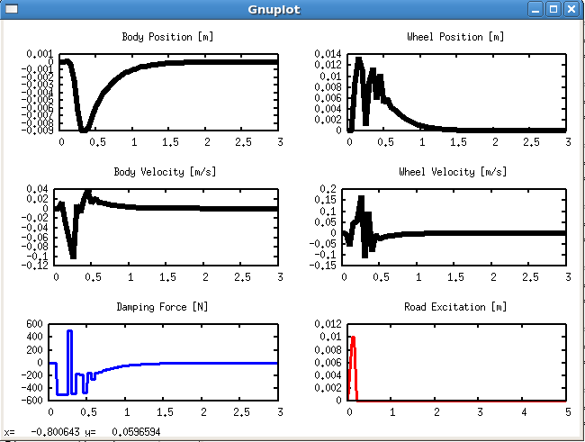
Here, we have simulated the road disturbance, which is displayed in the lower right part of the Gnuplot. Due to the "bump" in the road we observe an excitation of the body and the wheel, which is however quickly regulated back to zero, by the MPC controller. In addition, the control constraints on the damping force have been satisfied.

Next example: Using Grids and VariablesGrids