Setting-Up a Process for MPC Simulations

Table of Contents

• A Guiding Example: Simulation of a Quarter Car
• Basic Implementation of a Process for MPC Simulations in ACADO
• Obtaining the Simulation Results

This tutorial explains how to setup a simple Process for MPC simulations. As a guiding example, we consider a simple actively damped quarter car model.

A Guiding Example: Simulation of a Quarter Car

In this section we consider a first principle quarter car model with active suspension. The four differential states of this model xB , vB , xW , and vW are the position/velocity of the body/wheel, respectively. Our control input is a limited damping force F acting between the body and the wheel. The road, denoted by the variable R , is considered as an (unknown) external disturbance. The dynamic equations have the following form:

Within our simulation, we start at xB = 0.01 and all other states at zero. Moreover, we treat the mass of the body mB as manipulatable (time-constant) parameter, whereas fixed values are assigned to all other quantities.

In order to illustrate the concept, let us assume that not all states can be measured directly but only the first one together with a combination of the third one and the control input. For realizing this, we introduce the following output function:

Basic Implementation of a Process for MPC Simulations in ACADO

The following piece of code shows how to implement a Process simulation based on this quarter car model. It comprises four main steps:

1. Introducing all variables and constants.
2. Setting up the quarter car ODE model together with the output function; these two functions form the DynamicSystem used for the Process simulation. (In case you do not define an output function, the Process output will be all differential states.)
3. Setting up the Process, which comprises at least to define a dynamic system to be used for simulation together with the information which integrator is to be used. In our example, also integrator options are set, initial values for the differential states are defined and a plot window is specified. As the dynamic system of the quarter car comprises an external disturbance, we also have to specify values for it. This is done by reading the disturbance data from the file "road.txt".
4. Simulating the Process by first initializing it, passing the start time of the simulation (otherwise simulation starts at 0.0), and second run it with given values for the control input and the parameter input. Afterwards, results can be obtained and are plotted according to the previously flushed plot window.

#include <acado_toolkit.hpp>
#include <include/acado_gnuplot/gnuplot_window.hpp>

int main( ) 
{  
    USING_NAMESPACE_ACADO


    // INTRODUCE THE VARIABLES:
    // -------------------------
    DifferentialState xB;
    DifferentialState xW;
    DifferentialState vB;
    DifferentialState vW;

    Disturbance R;
    Control F;

    Parameter mB;
    double mW = 50.0;
    double kS = 20000.0;
    double kT = 200000.0;


    // DEFINE THE DYNAMIC SYSTEM:
    // --------------------------
    DifferentialEquation f;

    f << dot(xB) == vB;
    f << dot(xW) == vW;
    f << dot(vB) == ( -kS*xB + kS*xW + F ) / mB;
    f << dot(vW) == (  kS*xB - (kT+kS)*xW + kT*R - F ) / mW;

    OutputFcn g;
    g << xB;
    g << 500.0*vB + F;

    DynamicSystem dynSys( f,g );


    // SETUP THE PROCESS:
    // ------------------
    Process myProcess;

    myProcess.setDynamicSystem( dynSys,INT_RK45 );
    myProcess.set( ABSOLUTE_TOLERANCE,1.0e-8 );

    Vector x0( 4 );
    x0.setZero( );
    x0( 0 ) = 0.01;

    myProcess.initializeStartValues( x0 );
    myProcess.setProcessDisturbance( "road.txt" );

    myProcess.set( PLOT_RESOLUTION,HIGH );

    GnuplotWindow window;
                window.addSubplot( xB, "Body Position [m]" );
                window.addSubplot( xW, "Wheel Position [m]" );
                window.addSubplot( vB, "Body Velocity [m/s]" );
                window.addSubplot( vW, "Wheel Velocity [m/s]" );

                window.addSubplot( F,"Damping Force [N]" );
                window.addSubplot( mB,"Body Mass [kg]" );
                window.addSubplot( R, "Road Disturbance" );
                window.addSubplot( g(0),"Output 1" );
                window.addSubplot( g(1),"Output 2" );

        myProcess << window;


    // SIMULATE AND GET THE RESULTS:
    // -----------------------------
    VariablesGrid u( 1,0.0,1.0,6 );

    u( 0,0 ) = 10.0;
    u( 1,0 ) = -200.0;
    u( 2,0 ) = 200.0;
    u( 3,0 ) = 0.0;
    u( 4,0 ) = 0.0;
    u( 5,0 ) = 0.0;

    Vector p( 1 );
    p(0) = 350.0;

    myProcess.init( 0.0 );
    myProcess.run( u,p );


    VariablesGrid xSim, ySim;

    myProcess.getLast( LOG_SIMULATED_DIFFERENTIAL_STATES,xSim );
    xSim.print( "Simulated Differential States" );

    myProcess.getLast( LOG_PROCESS_OUTPUT,ySim );
    ySim.print( "Process Output" );

    return 0;
}

The file "road.txt" containing the disturbance data:

DATA FILE: road.txt

------------------------------

TIME      W

0.0       0.00
0.1       0.01
0.15      0.01
0.2       0.00
5.0       0.00

------------------------------

If we run the above piece of code in ACADO, the corresponding Gnuplot output should be as follows:

Simulation results

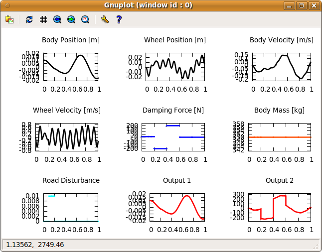
Note that this is only a simulation with user-specified control inputs; no feedback control is applied.

Obtaining the Simulation Results

We end this tutorial with proving a list of all results that can be obtained from the Process after simulation:

Logging Name:	Short Description:
LOG_PROCESS_OUTPUT	All process outputs as specified via the output function
LOG_SIMULATED_DIFFERENTIAL_STATES	All differential states as simulated within the Process
LOG_SIMULATED_ALGEBRAIC_STATES	All algebraic states as simulated within the Process
LOG_SIMULATED_CONTROLS	All control inputs as simulated within the Process
LOG_SIMULATED_PARAMETERS	All parameter inputs as simulated within the Process
LOG_SIMULATED_DISTURBANCES	All external disturbances as simulated within the Process
LOG_NOMINAL_CONTROLS	All nominal control inputs as given to the Process
LOG_NOMINAL_PARAMETERS	All nominal parameter inputs as given to the Process

Next example: Advanced Features for Simulating a Process