A State and Parameter Estimation Tutorial

Table of Contents

• Mathematical Formulation of the Optimization Problem:
• Implementation of the State and Parameter Estimation Problem with ACADO Toolkit:
• A brief discussion of the results:
• A posteriori analysis:
• Literature:

This tutorial explains how to setup a simple parameter estimation problem with ACADO. As an example a very simple pendulum model is considered. The aim is to estimate the length of the cable as well as a friction coefficient from a measurent of the excitation of the pendulum at several time points.

Mathematical Formulation of the Optimization Problem:

We consider a very simple pendulum model with two differential states φ and ω representing the excitation angle and the corresponding angular velocity of the pendulum respectively. Moreover, the model for the pendulum depends on two parameters: the length of the cable is denoted by l while the friction coefficient of the pendulum is denoted by α . The parameter estimation problem of our interest has now the following form:

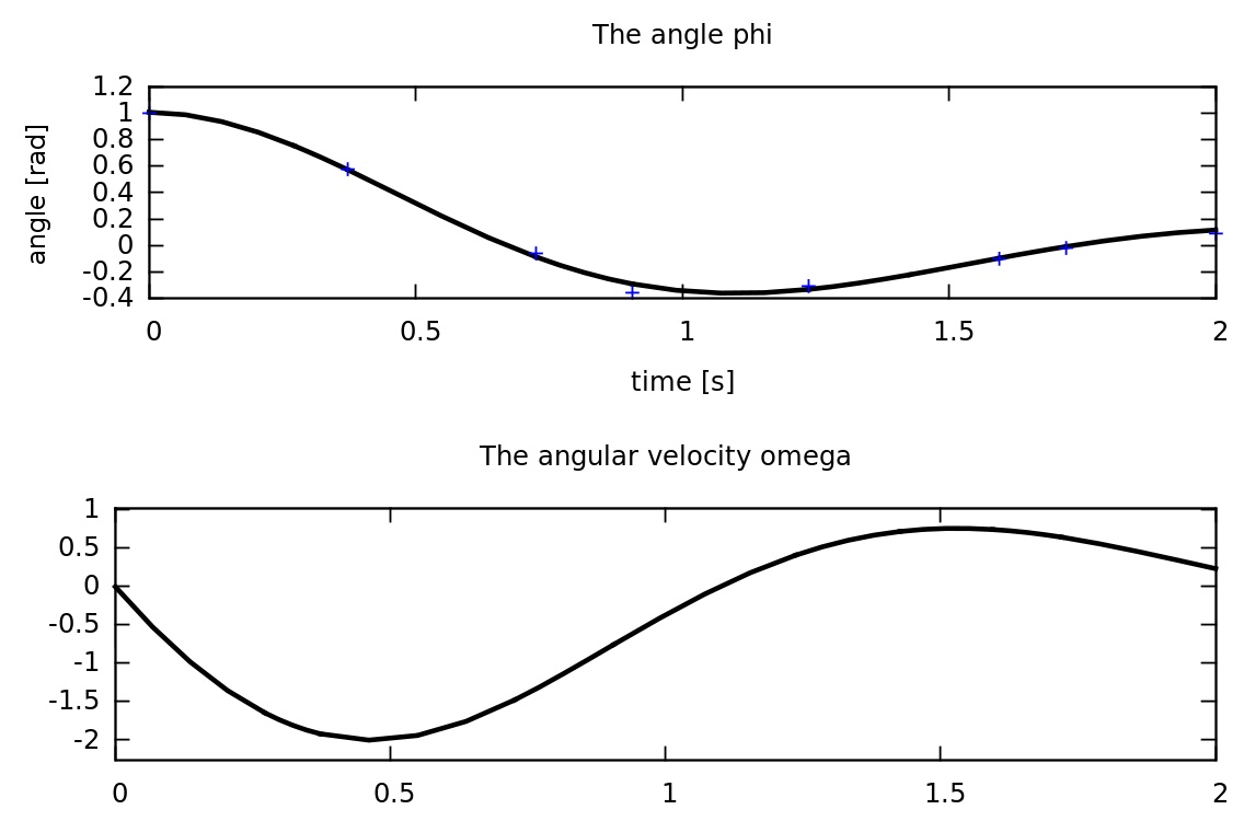
Here, we assume that the state φ has been measured at 10 points in time which are denoted by t1, ..., t10 while the corresponding measurement values are η1, ..., η10 . Note that the above formulation does not only regard the parameters l and α as free variables. The initial values of two states φ and ω are also assumed to be unknown and must be estimated from the measurements, too.

Implementation of the State and Parameter Estimation Problem with ACADO Toolkit:

The implementation of the above optimization problem is similar to the standard optimal control problem implementation which has been discussed in the tutorial "Time Optimal Control of a Rocket Flight". However, the main difference is now that the measurements have to be provided and that objective has a special least-squares form:

#include <acado_toolkit.hpp>
#include <include/acado_gnuplot/gnuplot_window.hpp>

int main( )
{
        USING_NAMESPACE_ACADO
        
        DifferentialState          phi, omega;    // the states of the pendulum
        Parameter                  l, alpha  ;    // its length and the friction
        const double               g = 9.81  ;    // the gravitational constant
        DifferentialEquation       f         ;    // the model equations
        Function                   h         ;    // the measurement function
        
        VariablesGrid measurements;                 // read the measurements
        measurements = readFromFile( "data.txt" );  // from a file.
        
        //  --------------------------------------
        OCP ocp(measurements.getTimePoints());    // construct an OCP
        h << phi                             ;    // the state phi is measured
        ocp.minimizeLSQ( h, measurements )   ;    // fit h to the data
        
        f << dot(phi  ) == omega             ;    // a symbolic implementation
        f << dot(omega) == -(g/l) *sin(phi )      // of the model
                                         - alpha*omega     ;    // equations
        
        ocp.subjectTo( f                    );    // solve OCP s.t. the model,
        ocp.subjectTo( 0.0 <= alpha <= 4.0  );    // the bounds on alpha
        ocp.subjectTo( 0.0 <=   l   <= 2.0  );    // and the bounds on l.
        //  --------------------------------------
        
        GnuplotWindow window;
        window.addSubplot( phi  , "The angle phi", "time [s]", "angle [rad]" );
        window.addSubplot( omega, "The angular velocity dphi"                );
        window.addData( 0, measurements(0) );
        
        //  --------------------------------------
        ParameterEstimationAlgorithm algorithm(ocp); // the parameter estimation
        algorithm << window;
        algorithm.solve();                           // solves the problem
        
        return 0;
}

Note that the measurement are in this example provided in form of the text file "data.txt" which has the following contents:

The file "data.txt"

TIME POINTS    MEASUREMENT OF PHI
-----------    ------------------
0.00000e+00    1.00000e+00
2.72321e-01    nan
3.72821e-01    5.75146e-01
7.25752e-01   -5.91794e-02
9.06107e-01   -3.54347e-01
1.23651e+00   -3.03056e-01
1.42619e+00    nan
1.59469e+00   -9.64208e-02
1.72029e+00   -1.97671e-02
2.00000e+00    9.35138e-02
---------------------------------    

At two time points the measurement was not successful leading to "nan" entries in the data file. In addition, the time points at which the measurements have been taken are not equidistant. Note that ACADO detects automatically the number of valid measurements in the file. Moreover, it is not necessary to specify any dimensions while the initialization is auto-generated, too.

A brief discussion of the results:

The parameter estimation algorithm chooses by default a Gauss Newton method. Running the above piece of code leads to the following output:

Output on the terminal:

#:    KKT tol.   Obj. Value    
---------------------------    
1:   1.564e+00   7.8507e-01    
2:   1.185e-03   3.1263e-03    
3:   8.172e-05   3.2632e-03    
4:   1.198e-07   3.2837e-03    
---------------------------    
                                                           
convergence achieved.

Note that the algorithm converges rapidly within 4 iterations as expected for a Gauss-Newton method. Recall that the Gauss-Newton method works very well for least-squares problem, where either the problem is almost linear or the least-squares residuum is small.

A posteriori analysis:

Once we are able to solve the parameter estimation we are usually interested in the results for the parameters. In addition, variance-covariance information about the quality of the fit is avaliable. A typical piece of code to get the output is as follows:

#include <acado_toolkit.hpp>
#include <include/acado_gnuplot/gnuplot_window.hpp>

int main( )
{
        USING_NAMESPACE_ACADO
        
        
        // ... (IMPLEMENTATION OF THE OCP AS ABOVE) ...
        
        
        ParameterEstimationAlgorithm algorithm(ocp);
        algorithm.solve();
        
        
        // GET THE OPTIMAL PARAMETERS:
        // ---------------------------
        VariablesGrid params;
        algorithm.getParameters( params );
        
        // GET THE VARIANCE COVARIANCE IN THE SOLUTION:
        // --------------------------------------------
        Matrix var;
        algorithm.getParameterVarianceCovariance( var );
        
        
        // PRINT THE RESULT ON THE TERMINAL:
        // ---------------------------------
        printf("\n\nResults for the parameters: \n");
        printf("-----------------------------------------------\n");
        printf("  l      =  %.3e +/- %.3e \n", params(0,0), sqrt( var(0,0) ) );
        printf("  alpha  =  %.3e +/- %.3e \n", params(0,1), sqrt( var(1,1) ) );
        printf("-----------------------------------------------\n\n\n");
        
        return 0;
}

Running the above piece of code leads to the common output for the results of a parameter estimation problem:

Results for the parameters: 
-----------------------------------------------    
   l      =  1.001e+00 +/- 1.734e-01
   alpha  =  1.847e+00 +/- 4.059e-01
-----------------------------------------------    

Note that the computation of the variance covariance matrix is based on a linear approximation in the optimal solution. The details of this strategy have originally been published by Bock [1].

Literature:

[1] H.G. Bock. Recent advances in parameter identification techniques for ODE. In P. Deuflhard and E. Hairer, editors, Numerical Treatment of Inverse Problems in Differential and Integral Equations. Birkhaeuser, Boston, 1983.

Next example: Setting-Up a Process for MPC Simulations