Table of Contents
This tutorial explains how to solve optimal control problems for which the model equation contains not only differential, but also algebraic states.
Mathematical formulation of general DAE optimization problems
For the general DAE formulation we summarize the differential and algebraic states of the DAE in one vector x . Moreover, we denote by u the control input, by p a constant parameter, and by T the time horizon length of an DAE optimization problem. The general problem formulation reads now as follows:
![\begin{eqnarray*} \displaystyle\min_{x(\cdot), u(\cdot), p, T} & \Phi(x(\cdot), u(\cdot), p, T) \\ \textrm{subject to} & \\ \forall t \in [0,T]: & 0 = F(t, x(t), \dot{x}(t), u(t), p), \\ \forall t \in [0,T]: & 0 \leq h(t, x(t), u(t), p), \\ & 0 = r(x(0), x(T), p)\\ \end{eqnarray*}](form_51.png)
Here, the function F denotes the model equation, Φ the objective functional, h the path constraints, and r the boundary constraints of the optimization problem.
Remarks:
- The model function F can in practice often be written as
In this case, we say that the DAE is semi-implicit.![\[ 0 = F(t, x(t), \dot{x}(t), u(t), p) = \left( \begin{array}{c} \dot{x}(t) - f_1(t,x(t),u(t),p) \\ f_2(t,x(t),u(t),p) \end{array} \right) \]](form_52.png)
- Another special case, which often occurs in practice, is that the function F is linear in dx/dt such that we have
for a matrix valued function M. However, in ACADO linear dependencies are automatically detected such that from the user point of view, we do not have to make a difference between linear and fully-implicit DAEs.![\[ 0 = F(t, x(t), \dot{x}(t), u(t), p) = M(t, x(t), u(t), p)\dot{x}(t) - f(t,x(t),u(t),p) \]](form_53.png)
An ACADO tutorial code for semi-implicit DAEs
The following piece of code illustrates how to setup a simple DAE optimization problem for the case that the DAE is semi-implicit:
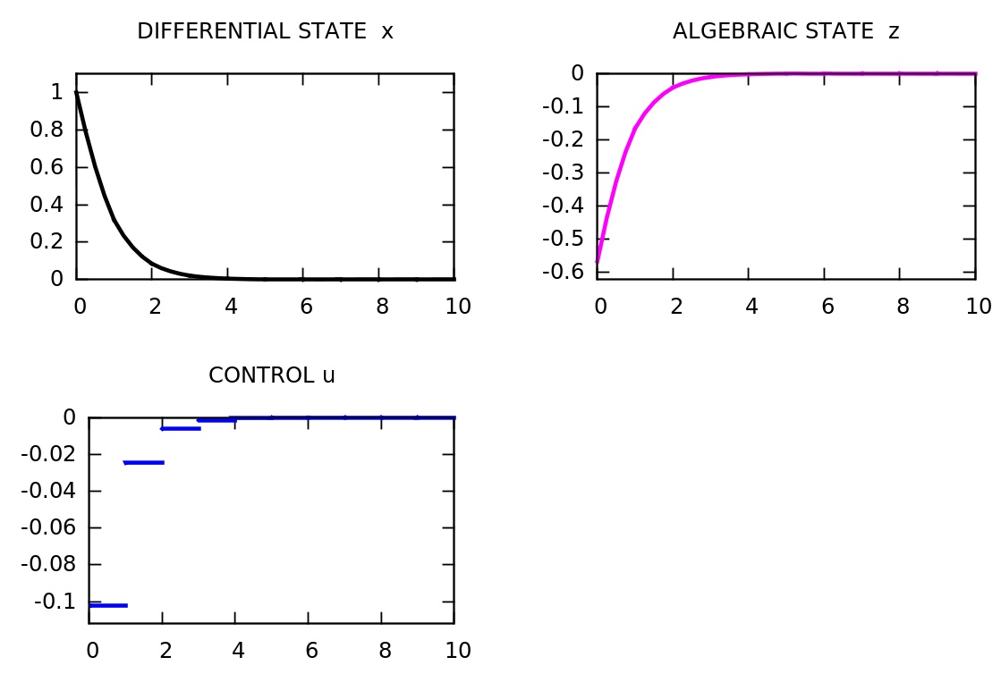
Running this example, the corresponding Gnuplot output should look as follows:
DAE optimization options for advanced users
work in progress
Next example: Optimal Control of Discrete-Time Systems