Plotting Results

The ACADO Toolkit allows to conveniently setup PlotWindows for plotting results with external packages (GNUplot by default). This tutorial explains how to use them.

Plotting Symbolic Quantities

All symbolic quantities like DifferentialStates, Controls etc. can be directly added to a PlotWindow. These PlotWindows can then be passed to an OptimizationAlgorithm which will take care that the desired quantities are plotted. We illustrate this based on a simple OCP formulation:

#include <acado_optimal_control.hpp>
#include <include/acado_gnuplot/gnuplot_window.hpp>

int main( )
{
    USING_NAMESPACE_ACADO

    // DEFINE SAMPLE OCP
    // -----------------
    DifferentialState x, y;
    Control           u;

    DifferentialEquation f;
    
    f << dot(x) == y;
    f << dot(y) == u;

    OCP ocp( 0.0, 5.0 );
    ocp.minimizeLagrangeTerm( x*x + 0.01*u*u );

    ocp.subjectTo( f );
    ocp.subjectTo( AT_START, x ==  1.0 );
    ocp.subjectTo( AT_START, y ==  0.0 );

    ocp.subjectTo( -1.0 <= u <=  1.0 );


    // SETUP OPTIMIZATION ALGORITHM AND DEFINE VARIOUS PLOT WINDOWS
    // ------------------------------------------------------------
    OptimizationAlgorithm algorithm( ocp );

    GnuplotWindow window1;
    window1.addSubplot( x, "1st state" );
    window1.addSubplot( y, "2nd state","x label","y label",PM_POINTS );
    window1.addSubplot( u, "control","x label","y label",PM_LINES,0,5,-2,2 );
    window1.addSubplot( 2.0*sin(x)+y*u, "Why not plotting fancy stuff!?" );
    
    GnuplotWindow window2( PLOT_AT_EACH_ITERATION );
    window2.addSubplot( x, "1st state evolving..." );
    
    algorithm << window1;
    algorithm << window2;
    
    algorithm.solve( );

    return 0;
}

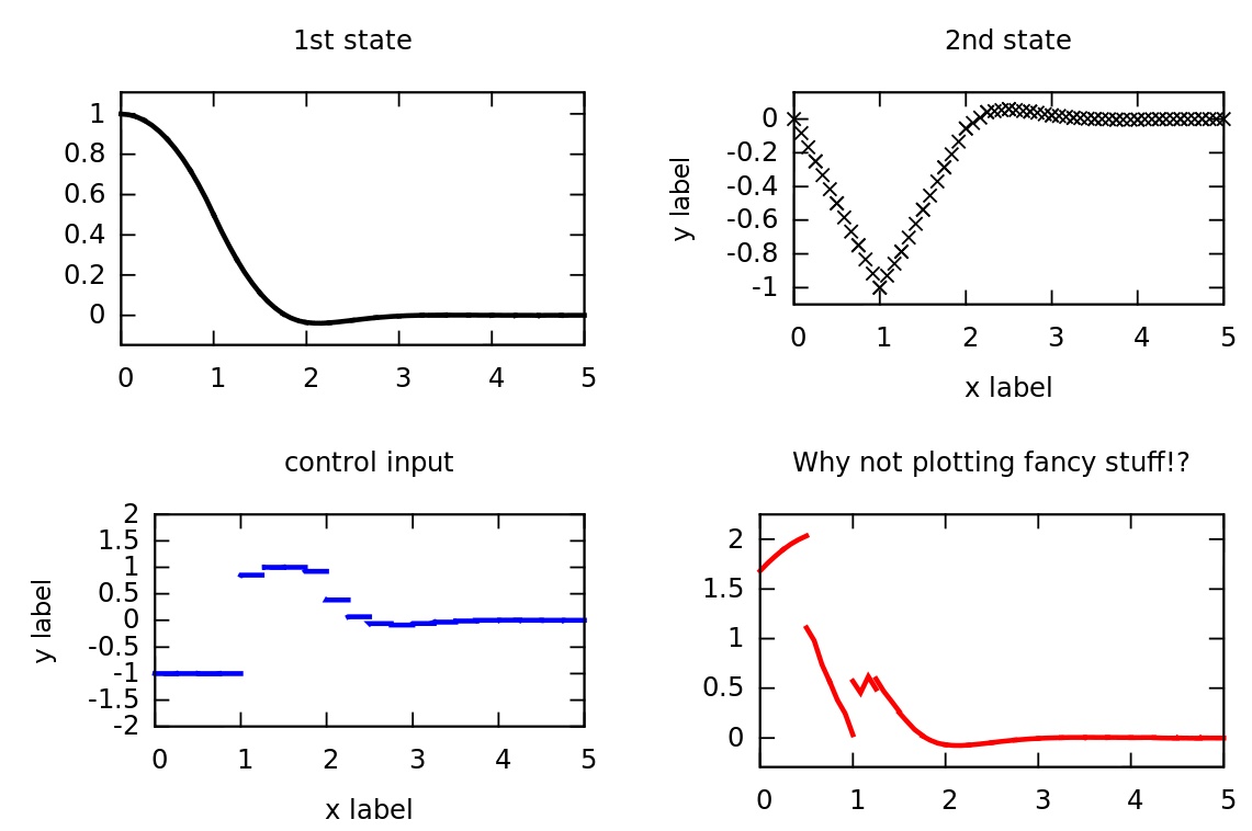
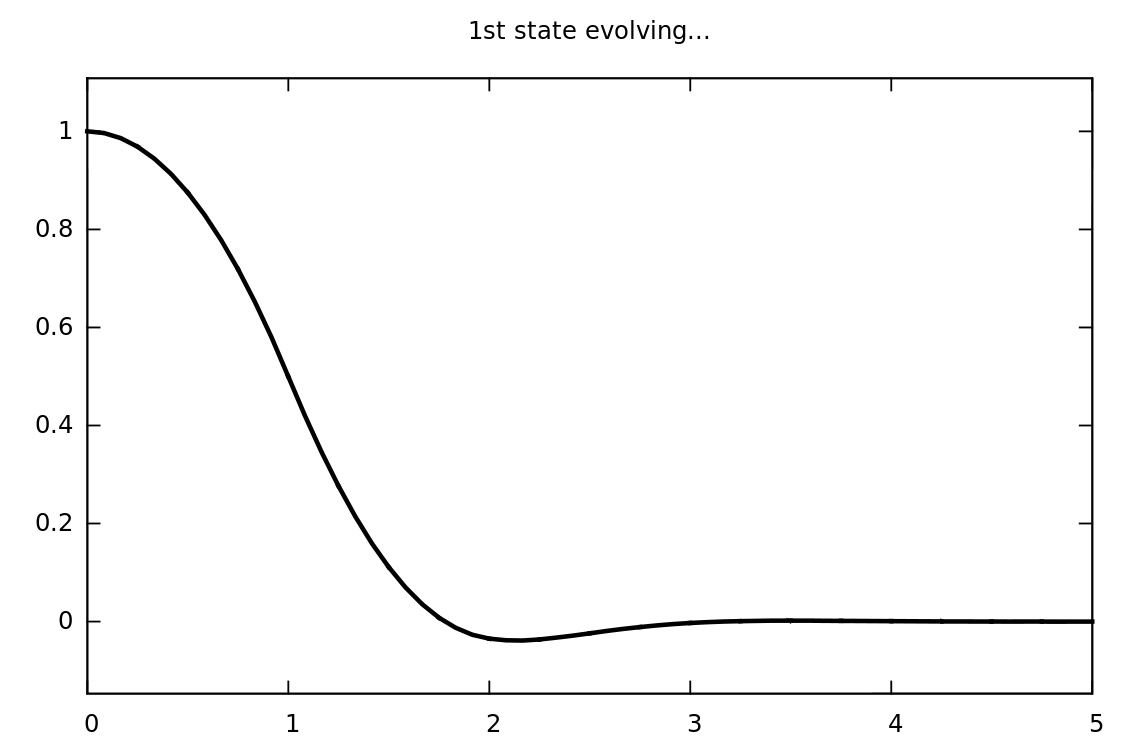
Having defined a simple OCP comprising the differential states "x" and "y" as well as a control "u", an OptimizationAlgorithm is set up. Afterwards, two plot windows are defined and flushed to the OptimizationAlgorithm before running it. In our example, two GnuplotWindows are instantiated that allow to use Gnuplot for plotting (make sure that the corresponding header file "gnuplot_window.hpp" is included as). By default, each plot window only plot the desired information at the end of the solution procedure. However, also one of the following option might be specified:

PlotFrequency:	Description:
PLOT_AT_START	Plot once after initialization of the algorithm
PLOT_AT_END	Plot once after termination of the algorithm
PLOT_AT_EACH_ITERATION	Plot after each iteration of the algorithm
PLOT_IN_ANY_CASE	Plot at start, at end and at each iteration
PLOT_NEVER	Do not plot at all

To each PlotWindow, an arbitrary number of subplots can be added using the "addSubplot" command. Only the first argument specifying the symbolic quantity to be plotted is mandatory. This might be followed by three strings specifying the title as well as the lables of the x and y axis of the subplots, respectively. Moreover, the fifth argument may specify whether the plotted data points are to be connected by lines (PM_LINES, default value) or not (PM_POINTS). Finally, arguments six to ten might specify the lower/upper limit of the x and the y axis, respectively. Each symbolic quantity is plotted with a pre-defined color depending on its type. At termination of the optimization algorithm, the two Gnuplot windows should look as follows:

Simulation results

Simulation results

Plotting VariablesGrids

Also arbitrary one-dimensional VariablesGrids can be plotted in very similar way as symbolic quantities. The only difference is that the user provides the respective data; the OptimizationAlgorithm can only collect data of symbolic quantaties automatically. Thus, flushing a plot window comprising a user-defined VariablesGrid to an OptimizationAlgorithm is of limited use. Instead, the user should rather directly call the "plot" command for plotting the plot window, as done the following example: Again, we first explain how to setup an equidistant VariablesGrid:

#include <acado_optimal_control.hpp>
#include <include/acado_gnuplot/gnuplot_window.hpp>

int main( )
{
    USING_NAMESPACE_ACADO

    VariablesGrid data( 1, 0.0,10.0,11 );
    data.setZero();
    data( 2,0 ) = 1.0;
    data( 5,0 ) = -1.0;
    data( 8,0 ) = 2.0;
    data( 9,0 ) = 2.0;

    // optionally, change type to adjust plot format
    // data.setType( VT_CONTROL );

    GnuplotWindow window;
    window.addSubplot( data, "Any data can be plotted" );
    window.plot();

    return 0;
}

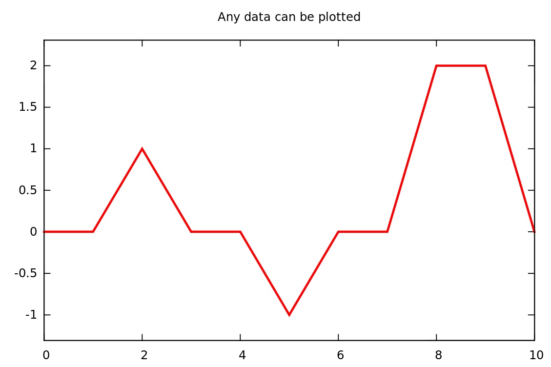
Running this example should result in the following Gnuplot window:

Simulation results

The default color for plotting user-defined VariablesGrids is red (it can be changed indirectly using the "setType" command).

Plotting Algorithmic Information

Work in progress...

Next example: Simulation of a Dynamic System