Advanced Features for Simulating a Process

This tutorial introduces more advanced features of the ACADO Process for MPC simulations. In particular, actuator and sensor behaviour can be simulated to yield more realistic results.

Adding a Actuator to the Process

Actuator effects can be simulated by adding an Actuator block to the Process as demonstrated in the following code fragment:

        // to be added to code fragment from previous Online Tutorial ...
        
        // SETUP NOISE:
        // ------------
        Vector mean( 1 ), amplitude( 1 );
        mean.setZero( );
        amplitude.setAll( 50.0 );
        
        GaussianNoise myNoise( mean,amplitude );
        
        
        // SETUP ACTUATOR:
        // ---------------
        Actuator myActuator( 1,1 );
        
        myActuator.setControlNoise( myNoise,0.1 );
        myActuator.setControlDeadTimes( 0.1 );
        
        myActuator.setParameterDeadTimes( 0.2 );
        
        // ...
        
        myProcess.setActuator( myActuator );

The code fragment shows how to setup a class generating one-dimensional, Gaussian noise with given amplitude (standard deviation) and mean. Afterwards, an Actuator accepting one control and one parameter input is defined. The previously defined noise will generated with a sampling time of 0.1 second and added to the control input. Moreover, both control and parameter inputs are delayed by the actuator by 0.1 and 0.2 seconds, respectively.

Adding a Sensor to the Process

Sensor effects can be simulated analogously by adding a Sensor block to the Process as demonstrated in the following code fragment:

        // to be added to code fragment from previous Online Tutorial ...
        
        // SETUP NOISE:
        // ---------------
        Vector mean( 1 ), amplitude( 1 );
        
        mean.setZero( );
        amplitude.setAll( 0.005 );
        UniformNoise myOutputNoise1( mean,amplitude );
        
        mean.setAll( 10.0 );
        amplitude.setAll( 50.0 );
        GaussianNoise myOutputNoise2( mean,amplitude );
        
        
        // SETUP SENSOR:
        // -------------
        Sensor mySensor( 2 );
        
        mySensor.setOutputNoise( 0,myOutputNoise1,0.1 );
        mySensor.setOutputNoise( 1,myOutputNoise2,0.1 );
        
        mySensor.setOutputDeadTimes( 0.2 );
        
        // ...
        
        myProcess.setSensor( mySensor );

In this code fragment, noise is setup that is to added to the process ouput. Two different instances of the noise class with different means and amplitudes are instantiated and assigned to the two components of the process output. Note that to the first component uniformly-distributed noise is added, while Gaussian noise is used for the second component in order to illustrate the flexibility of the concept. Finally, all output components are delayed by a dead time of 0.2 seconds.

Simulation Results

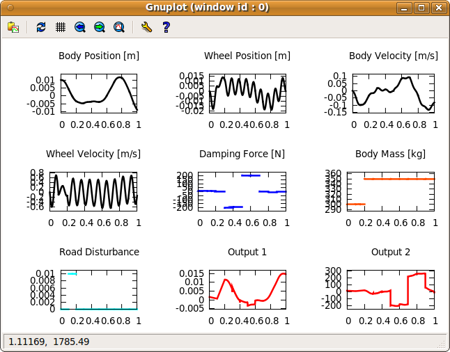
For completeness, we show the Gnuplot window of the quarter car process simulation from the previous Online Tutorial with the additions discussed before (and the parameter initialized at 300 to make the dead time visible):

Note that this is only a simulation with user-specified control inputs; no feedback control is applied.

List of Process Options

We end this tutorial with proving a list of the most common options that can be set when performing Process simulations:

Option Name:	Option Value:	Short Description:
INTEGRATOR_TOLERANCE	double	relative tolerance of the integrator
ABSOLUTE_TOLERANCE	double	absolute tolerance of the integrator ("ATOL")
MAX_NUM_INTEGRATOR_STEPS	int	maximum number of integrator steps
CONTROL_PLOTTING	PLOT_NOMINAL PLOT_REAL	specifying whether nominal or actual controls shall be plotted
PARAMETER_PLOTTING	PLOT_NOMINAL PLOT_REAL	specifying whether nominal or actual parameters shall be plotted
OUTPUT_PLOTTING	PLOT_NOMINAL PLOT_REAL	specifying whether nominal or actual outputs shall be plotted
PLOT_RESOLUTION	LOW MEDIUM HIGH	specifying screen resolution when plotting

Next example: Setting-Up an MPC Controller