Datapoint Filters

In this section, the various filters which can be applied to the reading and reference point clouds before performing the ICP process.

As a reminder, datapoint filters can have several purposes:

• Removing noisy points which render the alignment of point clouds difficult.

• Removing redundant points so as to speed up alignment

• Adding descriptive information to the points such as a surface normal vector, or the direction from the point to the sensor.

Note that datapoint filters differ from outlier filters which appear further down the ICP chain and have a different purpose.

Libpointmatcher provides developers with a number of datapoint filters which process an input point cloud into an intermediate point cloud used in the alignment procedure. Filters function as independent modules that can and often are combined into chains. Sequential chains of datapoint filters can thus be adapted to the alignment problem at hand.

Filter Index

Down-sampling

1. Bounding Box Filter

2. Maximum Density Filter

3. Maximum Distance Filter (deprecated)

4. Minimum Distance Filter (deprecated)

5. Distance Limit Filter

6. Maximum Point Count Filter

7. Maximum Quantile on Axis Filter

8. Random Sampling Filter

9. Remove NaN Filter

10. Shadow Point Filter

11. Voxel Grid Filter (deprecated)

12. Octree Grid Filter

13. Normal Space Sampling (NSS) Filter

14. Covariance Sampling (CovS) Filter

15. Spectral Decomposition Filter (SpDF)

Descriptor Augmenting

1. Add Descriptor Filter

2. Observation Direction Filter

3. Surface Normal Filter

4. Orient Normals Filter

5. Sampling Surface Normal Filter

6. Simple Sensor Noise Filter

7. Saliency Filter

8. Fixed Step Sampling Filter

An Example Point Cloud View of an Appartment

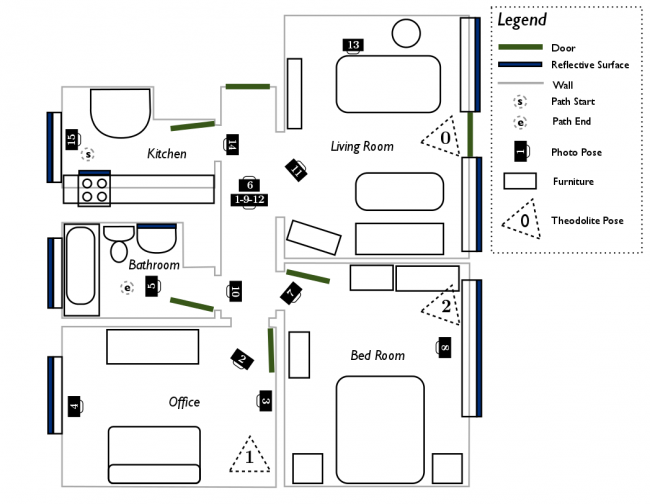
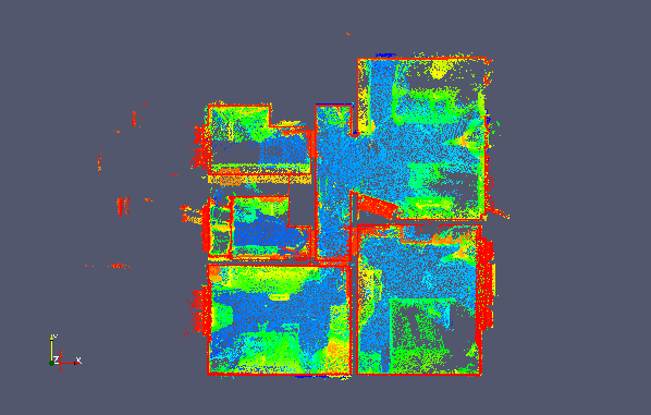
The following examples are drawn from the apartment dataset available for download from the ASL at ETH Zurich. A top-down view of the point cloud is depicted below, with the colors showing vertical elevation. The ceiling has been removed from the point cloud such that the floor (in blue) and the walls (in red) are clearly visible. Note that the coordinate origin is placed in the kitchen at the starting point of data capture, which is in the top-left of the top-down view and floor plan.

Add Descriptor Filter

Description

Adds a new descriptor to an existing point cloud or overwrites existing descriptor with the same name.

Required descriptors: none
Output descriptor: User defined.
Sensor assumed to be at the origin: no
Impact on the number of points: none
Altered descriptors: Existing descriptor with name equal to descriptorName.
Altered features: none.;

Parameter	Description	Default value	Allowable range
descriptorName	Name of the descriptor to be added.
descriptorDimension	Length of the descriptor to be added.	1	1 to 4294967295
descriptorValues	Values of the descriptor to be added. List of ‘descriptorDimension’ numbers of type T, separated by commas, closed in brackets, e.g. [2.2, 3.0, 6.1]

Bounding Box Filter

Description

Points can be excluded from a rectangular bounding region by using this filter. The box dimensions are specified by defining the maximum and minimum coordinate values in the x,y,z directions.

Required descriptors: none
Output descriptor: none
Sensor assumed to be at the origin: no
Impact on the number of points: reduces number of points

Parameter	Description	Default value	Allowable range
xMin	Minimum value on the x-axis defining one side of the box	-1.0	-inf to inf
xMax	Maximum value on the x-axis defining one side of the box	1.0	-inf to inf
yMin	Minimum value on the y-axis defining one side of the box	-1.0	-inf to inf
yMax	Maximum value on the y-axis defining one side of the box	1.0	-inf to inf
zMin	Minimum value on the z-axis defining one side of the box	-1.0	-inf to inf
zMax	Maximum value on the z-axis defining one side of the box	1.0	-inf to inf
removeInside	if set to 1, points contained within the box are removed, else points outside are removed	1	0 or 1

Example

In the following example, a box filter of the following dimensions was applied to the input point cloud.

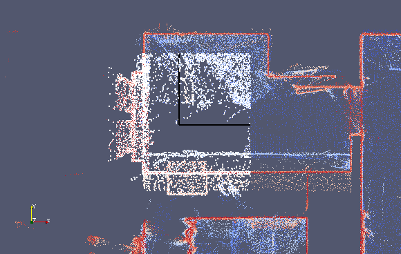
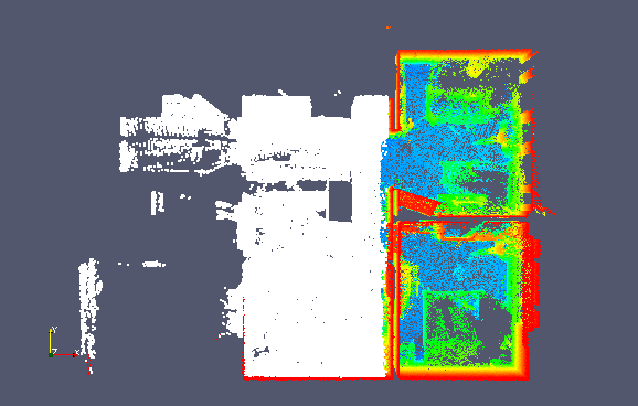
Note that only points outside the bounding box are removed by the filter by setting the property removeInside to 0. Because the point cloud center is located in the kitchen in the top-left, a square region of 2m x 2m is selected by this filter. In the following image, the output of the filter is overlaid in white.

Figure: Top down view of the appartment point cloud with a box filter applied. The input is shown in color and the output of the filter is overlaid in white	Parameters used
	xMin : -1.0 xMax : 1.0 yMin : -1.0 yMax : 1.0 zMin : -1.0 zMax : 2.0 removeInside : 0

Figure: Top down view of the appartment point cloud with a box filter applied. The input is shown in color and the output of the filter is overlaid in white	Parameters used
	xMin : -1.0 xMax : 1.0 yMin : -1.0 yMax : 1.0 zMin : -1.0 zMax : 2.0 removeInside : 1

Maximum Density Filter

Description

A number of filters are used to reduce the number of points in a cloud by randomly sub-sampling or randomly rejecting a set of points. Points in regions of high density often contain redundant information, and the ICP algorithm could be performed more efficiently with a smaller number of points. This filter is thus used to homogenize the density of a point cloud by rejecting a sub-sample of points in high-density regions.

Points are only considered for rejection if they exceed a density threshold, otherwise they are preserved. The single parameter of this filter sets the maximum density that should be obtained in the output point cloud. Points are randomly rejected such that this maximum density is obtained as closely as possible.

Required descriptors: densities (see SurfaceNormalDataPointsFilter and SamplingSurfaceNormalDataPointsFilter)
Output descriptor: none
Sensor assumed to be at the origin: no
Impact on the number of points: reduces number of points

Parameter	Description	Default value	Allowable range
maxDensity	The desired maximum density of points in points/m³ (for 3D), points/m² (for 2D)	10	min: 0.0000001, max: inf

Example

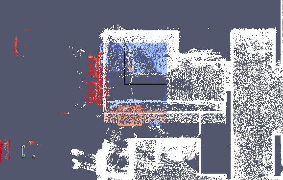
In the following example we observe the effect of the maximum density filter on the apartment point cloud. Sub-sampling occurs mostly in high density regions, which colored in red in the image below. The result is an image with lower density overall with the low density regions in blue being preserved.

Figure: Max density filter applied to subsection of the apartment dataset. On the original data, low density regions are blue and high density regions are red. The sampled points are overlaid in white.	Parameters used
	maxDensity: 50000

Maximum Distance Filter (deprecated)

Deprecated : please consider switching to Distance Limit Filter.

Description

These filters remove points which lie beyond a threshold distance from the coordinate center. Points are kept if their distance from the center is smaller than the threshold. The distance threshold can be defined on the x,y, and z axes or can be a radial distance from the center.

Required descriptors: none
Output descriptor: none
Sensor assumed to be at the origin: no
Impact on the number of points: reduces number of points

Parameter	Description	Default value	Allowable range
dim	Dimension over which the distance is thresholded. If -1, then the threshold is a radial distance from the center	-1	0: x, 1: y, 2: z, -1: radial
maxDist	Distance threshold (in m) beyond which points are rejected	1.0	min: -inf, max: inf

Example

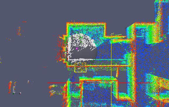
In the following example, a maximum distance threshold of 1m is applied radially by setting the dimension parameter to -1. As shown on the image below, points which lie within a sphere of radius 1m centered at the origin are selected by the filter and are displayed in white. All other points are rejected by the filter. Were a maximum distance filter to be replaced by an equivalent minimum distance filter, only points outside the sphere would be selected.

Figure: Max density filter applied to subsection of the apartment dataset. On the original data, low density regions are blue and high density regions are red. The sampled points are overlaid in white.	Parameters used
	maxDist : 1.0 dim : -1

Minimum Distance Filter (deprecated)

Deprecated : please consider switching to Distance Limit Filter.

Description

These filters remove points which lie beyond a threshold distance from the coordinate center. Points are kept if their distance from the center is greater than the threshold. The distance threshold can be defined on the x,y, and z axes or can be a radial distance from the center.

Required descriptors: none
Output descriptor: none
Sensor assumed to be at the origin: no
Impact on the number of points: reduces number of points

Parameter	Description	Default value	Allowable range
dim	Dimension over which the distance is thresholded. If -1, then the threshold is a radial distance from the center	-1	0: x, 1: y, 2: z, -1: radial
minDist	Distance threshold (in m) beyond which points are selected	1.0	min: -inf, max: inf

Distance Limit Filter

Description

These filters remove points which lie before or beyond a threshold distance from the coordinate center. The distance threshold can be defined on the x,y, and z axes or can be a radial distance from the center.

Required descriptors: none
Output descriptor: none
Sensor assumed to be at the origin: no
Impact on the number of points: reduces number of points

Parameter	Description	Default value	Allowable range
dim	Dimension over which the distance is thresholded. If -1, then the threshold is a radial distance from the center	-1	0: x, 1: y, 2: z, -1: radial
dist	Distance threshold (in m) used to reject points	1.0	min: -inf, max: inf
removeInside	If set to 1, points contained before the limit are removed, else points beyond are removed	1	0 or 1

Example

In the following example, a distance threshold of 1m is applied radially by setting the dimension parameter to -1. Also, the removeInside parameter is set to 0 in order to remove points beyond the distance limit. As shown on the image below, points which lie within a sphere of radius 1m centered at the origin are selected by the filter and are displayed in white. All other points are rejected by the filter. Were the removeInside parameter value to be replaced by 1, only points outside the sphere would be selected.

Figure: Distance limit filter applied to subsection of the apartment dataset. On the original data, low density regions are blue and high density regions are red. The sampled points are overlaid in white.	Parameters used
	dist : 1.0 dim : -1 removeInside : 0

Maximum Point Count Filter

Description

Conditional subsampling. This filter reduces the size of the point cloud by randomly dropping points if their number is above maxCount. The resulting point cloud while have maxCount number of point. the Based on: Registration and integration of multiple range images for 3-D model construction. Masuda, T. and Sakaue, K. and Yokoya, N. In Pattern Recognition, 1996., Proceedings of the 13th International Conference on. 879–883. 1996.

Required descriptors: none
Output descriptor: none
Sensor assumed to be at the origin: no
Impact on the number of points: reduces number of points

Parameter	Description	Default value	Allowable range
seed	srand seed	1	min: 0 max: 2147483647
maxCount	number of points beyond which subsampling occurs	1000	min: 0, max: 2147483647

Example

No example available.

Maximum Quantile on Axis Filter

Description

Points are filtered according to where they lie on a distribution of their positions along a given axis. The entire distance range is divided into quantiles which lie between 0 and 1. One can specify the distance quantile above or beneath which points are rejected by the filter.

Required descriptors: none
Output descriptor: none
Sensor assumed to be at the origin: no
Impact on the number of points: reduces number of points

Parameter	Description	Default value	Allowable range
dim	Dimension over which the distance (from the center) is thresholded	0	x:0 y:1 z:2
ratio	Quantile threshold. The threshold at which the points are rejected by the filter	0.5	min: 0.0000001, max: 0.9999999
removeBeyond	If 1 the points beyond the quantile threshold are rejected, else (0) the points under the quantile threshold are rejected	1	1 or 0

Example

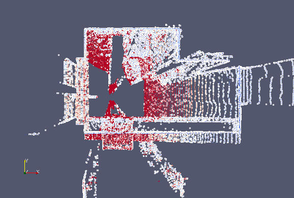
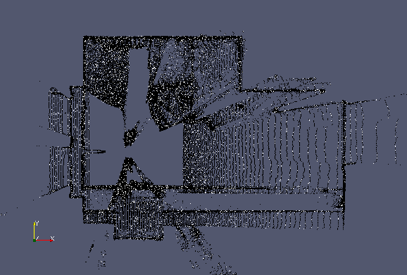
In the following example, maximum quantile filtering is performed over the x-axis with a quantile threshold of 0.5 and with the option to removeBeyond set to 1. Therefore, points which have an x-value which exceeds the 50% quantile are removed. The output of the filter is displayed in white and overlaid with the input point cloud in the image below. A sampling region centered at the origin and extending in both directions of the x-axis is clearly visible.

Figure: Maximum quantile on axis filter in the x-direction with a maximum quantile of 0.5 and removeBeyond set to 1.	Parameters used
	dim : 0 ratio : 0.5 removeBeyond : 1

Random Sampling Filter

Description

This filter behaves similarly to the Maximum Point Count Filter but does not enforce a maximum point constraint. Instead points are kept by the filter with a fixed probability.

Required descriptors: none
Output descriptor: none
Sensor assumed to be at the origin: no
Impact on the number of points: reduces number of points

Parameter	Description	Default value	Allowable range
prob	Probability that a point is kept (1/decimation factor)	0.75	min: 0, max: 1
randomSamplingMethod	Random sampling method: Direct RNG (0) (fastest), Uniform (1) (more accurate but slower)	0	min: 0, max: 1
seed	Seed for the random generator (-1 means no seed is used)	-1	min: -1, max: 2147483647

Example

In the following sample, points are kept with a probability of 0.1. Therefore the total number of points in the output point cloud is approximately 10 times less than the number of points in the input point cloud and the density is decreased overall.

Figure: After applying the random sampling filter with a probability of 0.1. The original data is shown in black and the sampled points in white.	Parameters used
	prob : 0.1

Remove NaN Filter

Description

Due to errors in the capture process point clouds may contain points with invalid coordinates. This filter can be applied to remove points which contain a NaN coordinate, thus producing a “clean” dataset.

Required descriptors: none
Output descriptor: none
Sensor assumed to be at the origin: no
Impact on the number of points: reduces number of points

Shadow Point Filter

Description

Shadow points are noisy points usually located at point cloud edge discontinuities.

Required descriptors: normals (see SurfaceNormalDataPointsFilter)
Output descriptor: none
Sensor assumed to be at the origin: no
Impact on the number of points: reduces number of points

IMPORTANT : The surface normal descriptors are required in the input point cloud.

Voxel Grid Filter (deprecated)

Deprecated : please, due to unefficient memory usage, consider switching to Octree Grid filter.

Description

While, the previous filters were sub-sampling filters in that they returned a sub-set of points from the original point cloud, the voxel grid filter instead returns a point cloud with a smaller number of points which should best represent the input point cloud as a whole.

The voxel grid filter down-samples the data by taking a spatial average of the points in the cloud. In the 2D case, one can simply imagine dividing the plane into a regular grid of rectangles. While the term is more suited to 3D spaces, these rectangular areas are known as voxels. The sub-sampling rate is adjusted by setting the voxel size along each dimension. The set of points which lie within the bounds of a voxel are assigned to that voxel and will be combined into one output point.

There are two options as to how to represent the distribution of points in a voxel by a single point. In the first, we take the centroid or spatial average of the point distribution. In the second, we simply take the geometrical center of the voxel. Clearly, the first option is more accurate since it takes into account the point distribution inside the voxels. However it is more computationally intensive since the centroid must be computed for each voxel. The computational cost increases linearly with the number of points in the cloud and the number of voxels.

This filter also provides two methods for sub-sampling descriptors. In the first, all descriptors within a voxel are averaged while in the second, only the first descriptor from a voxel is kept.

Required descriptors: none
Output descriptor: outputs average or single descriptor per voxel if the input cloud contains descriptors
Sensor assumed to be at the origin: no
Impact on the number of points: reduces number of points

Parameter	Description	Default value	Allowable range
vSizeX	Size of the voxel along the x-axis	1.0	]0 ; +inf[
vSizeY	Size of the voxel along the y-axis	1.0	]0 ; +inf[
vSizeZ	Size of the voxel along the z-axis	1.0	]0 ; +inf[
useCentroid	If 1, down-sample by using the centroid of each voxel. If 0, use the voxel center	1	1 or 0
averageExistingDescriptors	If 1, descriptors are down-sampled by taking their average in the voxel. If 0, we use the descriptors from the first point found in the voxel	1	1 or 0

For more information on the implementation of this filter, refer to this tutorial.

Example

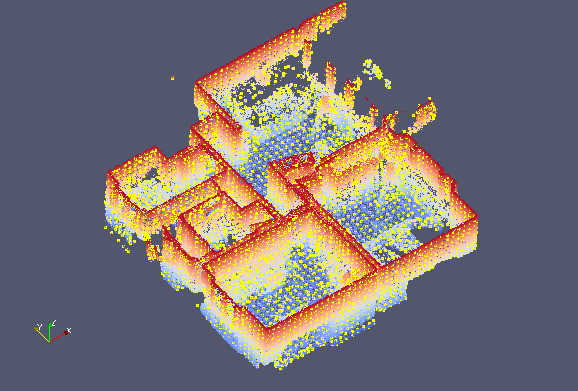
In this example, we apply the voxel grid filter using centroid down-sampling to the appartment point cloud. The output points are shown in yellow. You can observe a regular grid distribution of points corresponding to each voxel. A finer degree of sub-sampling can be obtained by using smaller voxels. This comes naturally with an increased computational cost and a larger output point cloud.

Figure: Applying the voxel grid filter filter to the appartment point cloud.	Parameters used
	vSizeX : 0.2 vSizeY : 0.2 vSizeZ : 0,2 useCentroid : 1

Octree Grid Filter

Description

The concept is quite the same as the voxel grid but use an Octree (3D case) or a Quadtree (2D case). The filter use the efficent spatial representation of the pointcloud by the octree to sub-sample point in each leaf.

Some information about the octree structure:

• the current implementation ensures to have either 0 or 8 (resp. 4) children for each node of the octree (resp. quadtree)

• only leaf nodes contain data

• data contained by the octree are currently the indexes of the points from the DataPoint structure

• processing are applied by calling a callback for each node in a depth-first search (DFS)

• parallel build can be enabled (but only the first level is parallelized)

• the octree can be build given two criterion: number of data by leaf node, or size of the leaf node

Remark 1: currently the space is decomposed from the Cartesian coordinates (x,y,z), but there should be no limitation to use other dimensions (such as normal coordinates for instance).

With this new structure, the DataPointsFilter named OctreeGridDataPointsFilter works as follow:

• build an octree spatial representation of the point cloud

• apply a process to sample in each leaf node

Four sampling methods are available:

• take the first point of each node (FirstPtsSampler)

• take a random point of each node (quite similar to the previous one since the point cloud is not supposed to be ordered) (RandomPtsSampler)

• compute centroid of each node (more precise but more costly) (CentroidSampler)

• compute medoid of each node (more precise but more costly) (MedoidSampler)

Remark 2: Theoretically, any process can be applied to the point cloud (sampling, feature enhancement, filtering, etc.) since the octree give an efficient spatial representation of the point cloud (ex: we could estimate the normal of each leaf).

Required descriptors: none
Output descriptor: none
Sensor assumed to be at the origin: no
Impact on the number of points: reduces number of points

Parameter	Description	Default value	Allowable range
buildParallel	flag for enabling parallel build of the octree	true (1)	0 or 1
maxPointByNode	number of point under which the octree stop dividing	1	min: 1, max: 4294967295
maxSizeByNode	size of the bounding box under which the octree stop dividing	0.0	min: 0.0, max: +inf
samplingMethod	method to sample the octree: First Point (0), Random (1), Centroid (2) (more accurate but costly), Medoid (3) (more accurate but costly)	0	min: 0, max: 3

Example

The following example uses a structured point cloud from the apartment dataset. As the pointcloud is structured we use the size criterion set to 20 cm to decompose the point cloud. In each leaf, we took the centroid (bottom) or the medoid (top) colored in green (output points), where the color of the pointcloud represents the indexes in the octree.

Figure: Applying the Octree Grid Filter on a structured point cloud	Parameters used
	maxSizeByNode : 0.2 at the top, samplingMethod : 3 (medoid) at the bottom, samplingMethod : 2 (centroid)

Remark 3: using centroid can lead to false results in the ICP registration. In deed, the centroid is not guaranteed to be a point of the cloud, which induce a new spatial representation and so an offset in the registration, whereas the medoid is by construction a point of the cloud. Both produce a similar sampled point cloud, but looking closer we can see that:

• In the top-right corner, sampled points are contained in the original point cloud

• In the bottom-right corner, sampled points are out of the point cloud.

Normal Space Sampling Filter

Description

Sub-sampling filter based on Normal Space Sampling (NSS) from S. Rusinkiewicz and M. Levoy, “Efficient Variants of the ICP Algorithm,” in Proceedings Third International Conference on 3-D Digital Imaging and Modeling, 2001, pp. 145–152.

The algorithm works as follow:

1. Construct a set of buckets in the normal-space (stocked in a std::vector)

2. Then put all points of the data into buckets based on their normal direction;

3. Finally, uniformly pick points from all the buckets until the desired number of points is selected.

Remark: a point is randomly picked in a bucket that contains multiple points.
Remark: the uniform sampling is based on a standard Mersenne twister engine

As the normals are supposed normed, the n-space can be represented by polar coordinates, with:

• theta, the polar angle in [0 ; pi]

• phi, the azimuthal angle in [0 ; 2pi]

• r=1, the radius can be omitted

Resources to better understand uniform sampling in normal-space can be found here.

Remark: the current implementation only supports 3D point cloud

Required descriptors: normals (see SurfaceNormalDataPointsFilter)
Output descriptor: none
Sensor assumed to be at the origin: no
Impact on the number of points: reduces number of points

Parameter	Description	Default value	Allowable range
nbSample	number of point to select	5000	min: 1, max: 4294967295
seed	seed for the random generator	1	min: 0, max: 4294967295
epsilon	step of discretization for the angle spaces	PI/32	min: PI/64, max: PI

Example

The following example uses a structured point cloud from the apartment dataset. The following gives the normal representation (on a sphere) of the original point cloud (we can clearly see that some areas are more populated) and the normal representation of the uniform sampled pointcloud (output).

Figure: Applying the NSS Filter on a structured point cloud	Parameters used
	nbSample : 5000 seed : 1 epsilon : PI/32

where the left-white point cloud is the normal distribution of the original point cloud, where the right-red point cloud is the normal distribution of the sampled point cloud

Covariance Sampling Filter

Description

Sub-sampling filter based on Covariance Sampling (CovS) from N. Gelfand, L. Ikemoto, S. Rusinkiewicz, and M. Levoy, “Geometrically stable sampling for the ICP algorithm,” in Fourth International Conference on 3-D Digital Imaging and Modeling, 2003. 3DIM 2003. Proceedings., 2003, pp. 260–267.

The filter analyses the force (t-normals: n) and the torque (r-normals: n x p) to select geometrically stable points that can bind the rotational components as well as the translational. Unlike the original article, we match the point-cloud with itself (considering then an overlap of 100%).

Three methods can be used to balance rotation and translation through torque normalization (L):

• L=1 (no normalization): more t-normals

• L=Lavg (average distance to centroid) : same contribution for t-normals and r-normals as torque is scale-independent

• L=Lmax (in unit ball): more r-normals

Required descriptors: normals (see SurfaceNormalDataPointsFilter)
Output descriptor: none
Sensor assumed to be at the origin: no
Impact on the number of points: reduces number of points

Parameter	Description	Default value	Allowable range
nbSample	number of point to select	5000	min: 1, max: 4294967295
torqueNorm	method for torque normalization: (0) L=1, (1) L=Lavg, (2) L=Lmax	1	min: 0, max: 2

Example

The following example uses a structured point cloud from the apartment dataset. The following gives the selected points (output) considering the three proposed normalization methods (L=1 in blue, L=Lavg in yellow and L=Lmax in red).

Figure: Applying the CovS Filter on a structured point cloud	Parameters used
	nbSample : 25000 torqueNorm : 0 (blue) 1 (yellow) 2 (red)

Remark: the filter is not very well suited for large scan with uneven density, it is preferably to use it for computer vision applications, or small scan.

Spectral Decomposition Filter (SpDF)

Description

Spectral Decomposition Filter (SpDF) is a sampling algorithm based on spectral decomposition analysis to derive local density measures for each geometric primitive. It is based on the reference Labussière, M., Laconte, J., & Pomerleau, F. (2020). Geometry Preserving Sampling Method Based on Spectral Decomposition for Large-Scale Environments. Frontiers in Robotics and AI, 7(September), 1–15. https://doi.org/10.3389/frobt.2020.572054

• First, we identify the geometric primitives along with their saliencies using the tensor voting framework.

• Then, we derive density measures from saliencies: if the density for each geometric primitive is less than the desired density, we stop; else we sub-sample each over-represented geometric primitive, and re-iterate.

• As output, we have a uniform sampled point cloud enhanced with geometric information.

Required descriptors: none
Output descriptor: normals, tangents, surfaceness, curveness, pointness, lambda1, lambda2, lambda3, sticks, plate, balls and labels (see SaliencyDataPointsFilter)
Sensor assumed to be at the origin: no
Impact on the number of points: make the density uniform, remove outliers, reduces number of points

Parameter	Description	Default value	Allowable range
k	Number of neighbors to consider	50	min: 6, max: 4294967295
sigma	Scale of the vote (in m) for the Tensor Voting framework	0.2	min: 0, max: +inf
radius	Radius to control the scale of the uniform distribution	0.4	min: 0, max: +inf
itMax	Number max of iterations to do	10	min: 1, max: 4294967295
keepNormals	Add the normal and tangent vectors to descriptors	1	1: true, 0: false
keepLabels	Add the labels (Surface = 3, Curve = 2, Junction = 1) to descriptors	1	1: true, 0: false
keepLambdas	Add the lambdas (saliencies of the tensor voting) to descriptors	1	1: true, 0: false
keepTensors	Add the tensors (stick, plate and ball tensors of the tensor voting) to descriptors	1	1: true, 0: false

Example

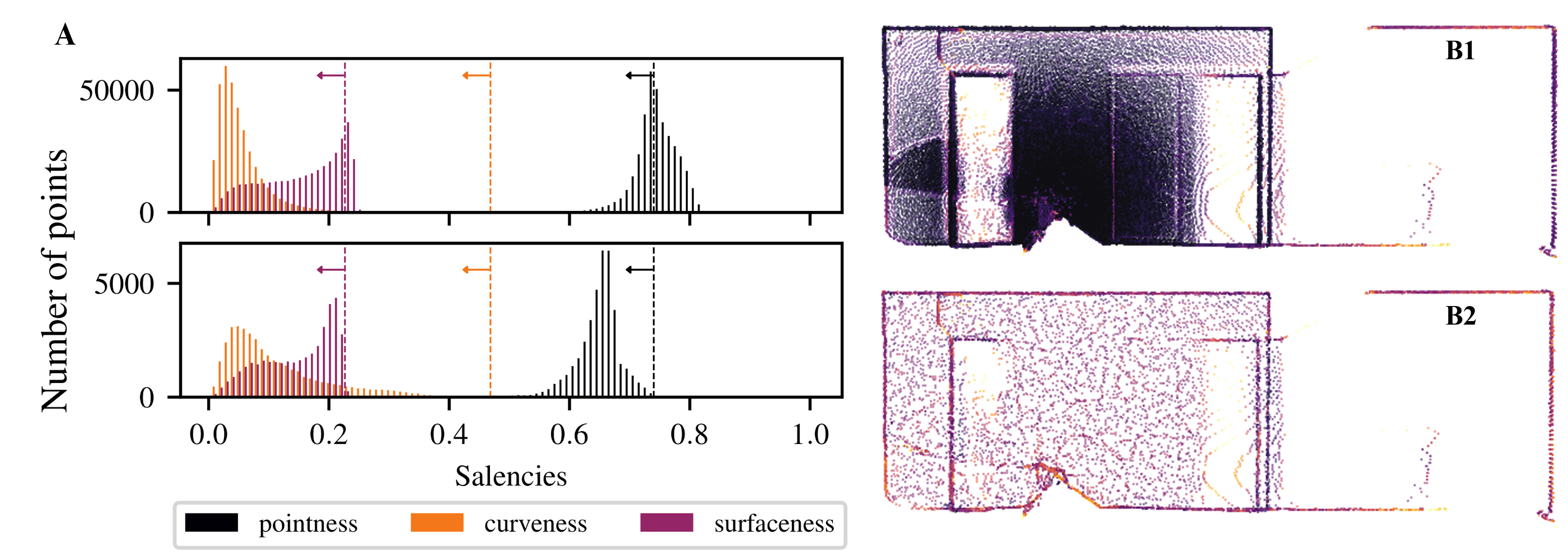
The figure bellow illustrates that SpDF is able to make the density uniform while preserving each geometric primitive, from an original point cloud of 370k points where most points are concentrated in a small area, to a uniform point cloud of 40k points, i.e., a compression ratio of 89%. Edges and corners have been preserved, while dense surfaces have been made uniform.

(A) shows the convergence of the saliencies below their expected values, represented by the vertical dashed lines, implying a uniform density on each geometric primitive. The top-histogram represents the initial saliencies distribution obtained from the tensor voting framework. The bottom-histogram shows the resulting distribution after making the density uniform.

(B) illustrates the process of reducing and making uniform a structured point cloud from 370k (B1) to 40k points (B2), i.e., a compression ratio of 89%. The resulting point cloud have uniform density, and geometric primitives, such as corners, edges and surfaces, are preserved.

Figure: Applying the SpDF Filter on a structured point cloud	Parameters used
	k : 50 sigma : 0.2 radius : 0.2

Observation Direction Filter

Description

As opposed to the previous filters, the following does not yield a sub-sample of points but rather augments the input point cloud with additional information. In particular, this filter adds a descriptor vector to each point representing its direction to the sensor used for capturing the point cloud. Remark that adding a direction vector is useful for locally captured point clouds in which the position of the sensor is fixed. In contrast global point clouds which are formed from several local point clouds do not have a fixed sensor position.

The returned direction vector is a vector connecting the point and the sensor, whose positions can be specified in the filter parameters.

Required descriptors: none
Output descriptor: observationDirections
Sensor assumed to be at the origin: yes
Impact on the number of points: none

Parameter	Description	Default value	Allowable range
x	x-coordinate of the sensor position	0.0	min: -inf, max: inf
y	y-coordinate of the sensor position	0.0	min: -inf, max: inf
z	z-coordinate of the sensor position	0.0	min: -inf, max: inf

Example

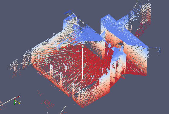
Remark: The following example uses a local point cloud 10 from the apartment dataset. The filter is used to extract direction informations and a small subset of these directions is shown in the following image. The arrows point towards the position of the sensor. The input point cloud is color coded according to the z-elevation of the points (red represents the ceiling and blue the floor).

Figure: Applying the observation direction filter to a local point cloud. A small subset of point observation directions are displayed	Parameters used
	x : 0 y : 0 z : 0

Surface Normal Filter

Description

The surface normal to each point is estimated by finding a number of neighboring points and taking the eigen-vector corresponding to the smallest eigen-value of all neighboring points.

Remark that that given a surface, the normal vector can point in two possible directions. Following the apartment example used herein throughout, the normal vector of a wall can point inside towards the room, or outside the apartment. To align all normal vectors in the same direction, the orient normals filter can be used.

Required descriptors: none
Output descriptor:
normals
densities
eigValues
eigVectors
Sensor assumed to be at the origin: no
Impact on the number of points: none

Parameter	Description	Default value	Allowable range
knn	Number of neighboring points (including the point itself) to consider when extracting surface normal	5	min: 3, max: 2147483647
epsilon	Approximation used in nearest neighbor search	0.0	min: 0.0, max: inf
keepNormals	Add the normal vector to descriptors	1	1: true, 0: false
keepDensities	Add point cloud density to descriptors	0	1: true, 0: false
keepEigenValues	Add eigen values to descriptors	0	1: true, 0: false
keepEigenVectors	Add eigen vectors to descriptors	0	1: true, 0: false
keepMatchedIds	Add identifiers of matched points to descriptors (see)	0	1: true, 0:false

Example

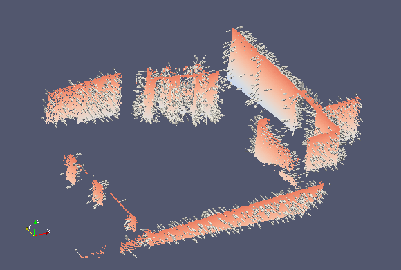
In this example, we again use a local point cloud of the apartment. You may recognize the input point cloud as a small portion of the local cloud used in the observation direction filter. The surface normals are extracted using 20 neighboring points and epsilon=0. In this example, for clarity, we only view a wall section of one of the apartment dataset. A random set of normal vectors is shown in the figure with arrows. When looking at the arrow directions on the wall, one may see normal vectors either pointing downwards into the apartment or outside the apartment.

Figure: Applying the observation direction filter to a local point cloud. A small subset of point observation directions are displayed	Parameters used
	knn : 20 epsilon : 0 keepNormals : 1 keepDensities : 1

Orient Normals Filter

Description

As explained previously, neighboring surface normal vectors obtained from the surface normals filter, do not have the same orientation. This filter enforces this constraint and reorients vectors from the same surface in a consistent direction. Vectors are reoriented to either point towards the center (inwards), or away from the center (outwards).

Required descriptors:
observationDirections (see ObservationDirectionDataPointsFilter)
normals (see SurfaceNormalDataPointsFilter and SamplingSurfaceNormalDataPointsFilter)
Output descriptor: none
Sensor assumed to be at the origin: yes
Impact on the number of points: none

Parameter	Description	Default value	Allowable range
towardCenter	Orient vectors to point towards the center	1	1: true, 0: false

IMPORTANT : Both the normal vector descriptor and observation direction descriptors must be present in the input point cloud. Consequently, both the surface normal and observation filters should be applied prior to using this filter.

Example

The same input section is used as for extracting the surface normals in the previous section. The vectors are reoriented to point towards the center which lies in the bottom left corner of the image below. We now observe that adjacent surface normal vectors point in a consistent direction.

Figure: Normal vectors reoriented to point towards the center	Parameters used
	towardCenter: 1

Sampling Surface Normal Filter

Description

The above filters extract surface normals at every point in the point cloud. In point clouds representing planar surfaces however, a significant redundant information is contained in adjacent normal vectors. This filter attempts to both reduce the number of points within a point cloud and the number of different normal vectors. The first is achieved by performing either random sub-sampling as seen previously, or by using one point per box (bin sub-sampling). The latter is achieved by recursively decomposing the point-cloud space into boxes until each box contains at most knn points. A single normal vector is computed from the knn points in each box.

Required descriptors: none
Output descriptor:
normals
densities
eigValues
eigVectors
Sensor assumed to be at the origin: yes
Impact on the number of points: reduces number of points

Parameter	Description	Default value	Allowable range
ratio	Ratio of points (sampled randomly) that are preserved within a box	0.5	min: 0.0000001, max: 0.9999999
knn	Number of points contained within a box and number of neighboring points (including the point itself) to consider when extracting surface normal	7	min: 3, max: 2147483647
samplingMethod	0: random sub-sampling 1:bin sub-sampling with resulting number of points 1/knn	0	0 or 1
maxBoxDim	Maximum allowed length of a box above with boxes are discarded	inf	min: 0.0000001, max: inf
averageExistingDescriptors	Average existing descriptors within a box or keep existing values	1	0: keep existing 1: average existing
keepNormals	Add the normal vector to descriptors	1	1: true, 0: false
keepDensities	Add point cloud density to descriptors	0	1: true, 0: false
keepEigenValues	Add eigen values to descriptors	0	1: true, 0: false
keepEigenVectors	Add eigen vectors to descriptors	0	1: true, 0: false
keepMatchedIds	Add identifiers of matched points to descriptors	0	1: true, 0: false

Example

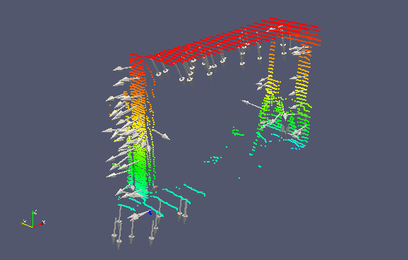
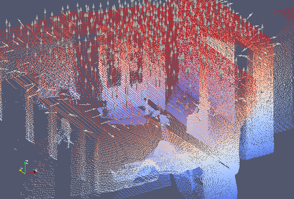
We reuse the same apartment section to illustrate the sampling of normal vectors. The decimation rate used is 0.5 such that half of the points from the original point cloud are discarded randomly. We use a knn value of 100 such that each box contains at most 100 points. In the following two figures, we extract sample points based on the normals and display the normal vectors at these sample points. We first do so for a ceiling section, followed by a ground section. Because the ceiling is essentially a large plane, the sampling is low and the normal vector arrows are dispersed relatively equally as shown in the first figure. On the other hand, the ground section has a higher density of points. This results in a denser sampling of points which is seen in the second figure.

The box centers are shown in red on the following picture. It is clear that as opposed to previous filters, adjacent points within a box have the same normal vector.

Figure: Sampled normal vectors of ceiling section	Parameters used
	knn : 100 ratio : 0.5 samplingMethod : 1

Figure: Sampled normal vectors ground section	Parameters used
	knn : 100 ratio : 0.5 samplingMethod : 1

Simple Sensor Noise Filter

Description

This filter is used to augment points with an estimation of position uncertainty based on sensor specifications. So far the SICK LMS, Hokuyo URG-04LX and UTM-30LX, as well as the Microsoft Kinect and Asus Xtion sensors are supported. The uncertainty or noise radius is represented in meters, and can be adjusted by varying a gain parameter which amplifies predefined uncertainty levels.

Required descriptors: none
Output descriptor: simpleSensorNoise
Sensor assumed to be at the origin: yes
Impact on the number of points: none

Parameter	Description	Default value	Allowable range
sensorType	The type of sensor that was used in the capture. 0: Sick LMS-1xx 1: Hokuyo URG-04LX 2 : Hokuyo UTM-30LX 3 : Kinect/Xtion	0	0, 1, 2, or 3
gain	Used to augment uncertainty	1	min: 1, max: inf

Example

For this example we use another point cloud dataset from the ASL collection called ETH Hauptgebaude. This dataset represents the main gallery of the main building at ETHZ and presents long straight corridors. We therefore use to display the uncertainty estimation of point clouds.

In the following image we show a side view of local point cloud 3 in the dataset. The laser is located at the bottom left corner and one can see the long arched corridor structures. As we move right in the image point are located further away from the sensor, are therefore less numerous and more uncertain. The points are colored by the estimation uncertainty obtained with this filter. More certain points are black, medium certain points are red and less curtain points are white. Naturally the colour shifts from black to white as we move further away from the laser down the corridor.

Figure: Side view of a view 3 from the HG dataset augmented with sensor noise estimations	Parameters used
	sensorType : 1

Saliency Filter

Description

This filter enhances the point cloud by computing geometric features saliencies throught the tensor voting framework. The implementation of the tensor voting is based on the closed-form solution of Wu, T.-P., Yeung, S.-K., Jia, J., Tang, C.-K., & Medioni, G. (2012). A Closed-Form Solution to Tensor Voting: Theory and Applications. IEEE Transactions on Pattern Analysis and Machine Intelligence, 34(8), 1482–1495. https://doi.org/10.1109/TPAMI.2011.250.

Required descriptors: none
Output descriptor: normals, tangents, surfaceness, curveness, pointness, sticks, plate, balls and labels
Sensor assumed to be at the origin: no
Impact on the number of points: none

Parameter	Description	Default value	Allowable range
k	Number of neighbors to consider	50	min: 6, max: 4294967295
sigma	Scale of the vote (in m) for the Tensor Voting framework	0.2	min: 0, max: +inf
keepNormals	Add the normal and tangent vectors to descriptors	1	1: true, 0: false
keepLabels	Add the labels (Surface = 3, Curve = 2, Junction = 1) to descriptors	1	1: true, 0: false
keepTensors	Add the tensors (stick, plate and ball tensors of the tensor voting) to descriptors	1	1: true, 0: false

Fixed Step Sampling Filter (To be completed)

The number of points in a point cloud can be reduced by taking random point subsamples. The filter is parametrized so that a fixed number of points - selected uniformly at random - are ‘rejected’ in the filtering process.

Where To Go From Here

This concludes the overview of data point filters. For a tutorial on writing a simple application for applying data point filters to an input point cloud, go here. To learn more about the general configuration of the ICP chain go here.