Calculate optimal switching time

Now let us calculate the optimal time to switch between the energy shaping swing-up controller and the linear feedback stabilizing controller. In order to determine this time, tools from optimal control are employed; however, the details of why these tools work is not explained here. The point is to show how trep facilitates the implementation because it has already precomputed all the necessary derivatives.

Create pendulum system

The code used to create the pendulum system and the controllers is identical to the previous sections, except a new variable has been added that designates the switching time. This is initially set to an initial guess equal to one-half the final time. We will then use this initial guess to find the optimal switching time. This variable is tau is highlighted in the code below.

import math
from math import pi
import numpy as np
from numpy import dot
import trep
import trep.discopt
from trep import tx, ty, tz, rx, ry, rz
import pylab

# Build a pendulum system
m = 1.0 # Mass of pendulum
l = 1.0 # Length of pendulum
q0 = 0. # Initial configuration of pendulum
t0 = 0.0 # Initial time
tf = 10.0 # Final time
dt = 0.01 # Sampling time
qBar = pi # Desired configuration
Qi = np.eye(2) # Cost weights for states
Ri = np.eye(1) # Cost weights for inputs
uMax = 5.0 # Max absolute input value
tau = 5.0 # Switching time

system = trep.System() # Initialize system

frames = [
    rx('theta', name="pendulumShoulder"), [
        tz(-l, name="pendulumArm", mass=m)]]
system.import_frames(frames) # Add frames

# Add forces to the system
trep.potentials.Gravity(system, (0, 0, -9.8)) # Add gravity
trep.forces.Damping(system, 1.0) # Add damping
trep.forces.ConfigForce(system, 'theta', 'theta-torque') # Add input

# Create and initialize the variational integrator
mvi = trep.MidpointVI(system)
mvi.initialize_from_configs(t0, np.array([q0]), t0+dt, np.array([q0]))

# Create discrete system
TVec = np.arange(t0, tf+dt, dt) # Initialize discrete time vector
dsys = trep.discopt.DSystem(mvi, TVec) # Initialize discrete system
xBar = dsys.build_state(qBar) # Create desired state configuration

# Design linear feedback controller
Qd = np.zeros((len(TVec), dsys.system.nQ)) # Initialize desired configuration trajectory
thetaIndex = dsys.system.get_config('theta').index # Find index of theta config variable
for i,t in enumerate(TVec):
    Qd[i, thetaIndex] = qBar # Set desired configuration trajectory
    (Xd, Ud) = dsys.build_trajectory(Qd) # Set desired state and input trajectory

Qk = lambda k: Qi # Create lambda function for state cost weights
Rk = lambda k: Ri # Create lambda function for input cost weights
KVec = dsys.calc_feedback_controller(Xd, Ud, Qk, Rk) # Solve for linear feedback controller gain
KStabilize = KVec[0] # Use only use first value to approximate infinite-horizon optimal controller gain

# Design energy shaping swing-up controller
system.get_config('theta').q = qBar
eBar = system.total_energy()
KEnergy = 1

Create cost

In order to perform an optimization anything there must be some sort of cost functional that is desirable to minimize. Trep has built in objects to deal with cost functions and that is what is used here.

cost = trep.discopt.DCost(Xd, Ud, Qi, Ri)

The cost object is created with the trep.discopt.DCost method, which takes in a state trajectory, input trajectory, state weighting matrix, and input weighting matrix.

In this case we used the same trajectories and weights that were used for the design of the linear feedback controller that stabilizes the pendulum to the upright unstable equilibrium.

Below is a list of the properties and methods of the cost class.

>>> cost.
cost.Q       cost.R       cost.l_du    cost.l_dx    cost.l_dxdx  cost.m_dx    cost.ud
cost.Qf      cost.l       cost.l_dudu  cost.l_dxdu  cost.m       cost.m_dxdx  cost.xd

Please refer to the Discrete Trajectory Cost documentation to learn more this object.

Angle utility functions

Since we would like the stabilizing controller to stabilize to any multiple of \(\pi\), two helper functions are used to wrap the angles to between \(0\) and \(2\pi\) and between \(-\pi\) and \(\pi\).

def wrapTo2Pi(ang):
    return ang % (2*pi)

def wrapToPi(ang):
    return (ang + pi) % (2*pi) - pi

Simulate function

The simulation of the system is done exactly the same way as in previous sections, except this time the forward simulation is wrapped into its own function. This makes running the optimization simpler because the simulate function can be called with different switching times instead of having to have multiple copies of the same code.

def simulateForward(tau, dsys, q0, xBar):
    mvi = dsys.varint
    tf = dsys.time[-1]

    # Reset discrete system state
    dsys.set(np.array([q0, 0.]), np.array([0.]), 0)

    # Initial conditions
    k = dsys.k
    t = dsys.time[k]
    q = mvi.q1
    x = dsys.xk
    fdx = dsys.fdx()
    xTilde = np.array([wrapToPi(x[0] - xBar[0]), x[1]])
    e = system.total_energy() # Get current energy of the system
    eTilde = e - eBar # Get difference between desired energy and current energy

    # Initial list variables
    K = [k] # List to hold discrete update count
    T = [t] # List to hold time values
    Q = [q] # List to hold configuration values
    X = [x] # List to hold state values
    Fdx = [fdx] # List to hold partial to x
    E = [e] # List to hold energy values
    U = [] # List to hold input values
    L = [] # List to hold cost values

    # Simulate the system forward
    while mvi.t1 < tf-dt:
        if mvi.t1 < tau:
            if x[1] == 0:
                u = np.array([uMax]) # Kick if necessary
            else:
                u = np.array([-x[1]*KEnergy*eTilde]) # Swing-up controller
        else:
            u = -dot(KStabilize, xTilde) # Stabilizing controller
        u = min(np.array([uMax]), max(np.array([-uMax]), u)) # Constrain input

        dsys.step(u) # Step the system forward by one time step

        # Update variables
        k = dsys.k
        t = TVec[k]
        q = mvi.q1
        x = dsys.xk
        fdx = dsys.fdx()
        xTilde = np.array([wrapToPi(x[0] - xBar[0]), x[1]])
        e = system.total_energy()
        eTilde = e - eBar
        l = cost.l(np.array([wrapTo2Pi(x[0]), x[1]]), u, k)

        # Append to lists
        K.append(k)
        T.append(t)
        Q.append(q)
        X.append(x)
        Fdx.append(fdx)
        E.append(e)
        U.append(u)
        L.append(l)

    J = np.sum(L)
    return (K, T, Q, X, Fdx, E, U, L, J)

The choice of which controller to use within the simulation function is decided based on if the simulation time is less than the switching time (highlighted above). If the simulation time is less than tau then the swing-up controller is used, otherwise the linear stabilizing controller is used. Also note that we store and return a vector of the derivatives of the dynamics with respect to the state (highlighted above) i.e. trep.discopt.DSystem.fdx.

Optimize

The optimization of the switching time is done in the standard way of using a gradient decent method to minimize a cost function with respect to the switching time. Both a descent direction and a step size must be calculated. The negative gradient of the cost to the switching time is used for the descent direction. Therefore, the switching time is updated with the following

\[\tau(k+1) = \tau(k) - \gamma*\frac{\partial J}{\partial \tau(k)}\]

where \(\tau\) is the switching time, \(\gamma\) is the step size, and \(J\) is the cost function.

To calculate the negative gradient in each iteration of the optimization, first the system is simulated forward from the initial time to the final time. Then the costate of the system is simulated backward from the final time to the switching time. The gradient at the switching time is the inner product of the difference between the two control laws and the costate.

Trep greatly simplifies this calculation because it has already calculated the necessary derivatives. In the simulation function the derivative of the system with respect to \(x\) (highlighted above) is stored at each time instance. Also, the derivative of the cost with respect to \(x\) has been already calculated with trep. Both of these derivatives are used in the backward simulation of the costate (highlighted below).

An Armijo line search is used to calculate the step size in each iteration of the optimization.

cnt = 0
Tau = []
JVec = []
JdTau = float('Inf')
while cnt < 10 and abs(JdTau) > .001:
    cnt = cnt + 1

    # Simulate forward from 0 to tf
    (K, T, Q, X, Fdx, E, U, L, J) = simulateForward(tau, dsys, q0, xBar)

    # Simulate backward from tf to tau
    k = K[-1]
    lam = np.array([[0],[0]])
    while T[k] > tau + dt/2:
       lamDx = np.array([cost.l_dx(X[k], U[k-1], k)])
       f2Dx = Fdx[k]
       lamDt = -lamDx.T - dot(f2Dx.T,lam)
       lam = lam - lamDt*dt
       k = k - 1

    # Calculate dynamics of swing-up controller at switching time
    x = X[k]
    xTilde = np.array([wrapToPi(x[0] - xBar[0]), x[1]])
    u1 = -dot(KStabilize, xTilde)
    u1 = min(np.array([uMax]), max(np.array([-uMax]), u1))
    dsys.set(X[k], u1, k)
    f1 = dsys.f()

    # Calculate dynamics of stabilizing controller at switching time
    eTilde = E[k] - eBar
    u2 = np.array([-x[1]*KEnergy*eTilde])
    u2 = min(np.array([uMax]), max(np.array([-uMax]), u2))
    dsys.set(X[k], u2, k)
    f2 = dsys.f()

    # Calculate value  of change in cost to change in switch time
    JdTau = dot(f1-f2, lam)

    # Armijo - used to determine step size
    chi = 0
    alpha = .5
    beta = .1
    tauTemp = tau - (alpha**chi)*JdTau
    (KTemp, TTemp, QTemp, XTemp, FdxTemp, ETemp, UTemp, LTemp, JTemp) = simulateForward(tauTemp, dsys, q0, xBar)
    while JTemp > J + (alpha**chi)*beta*(JdTau**2):
        tauTemp = tau - (alpha**chi)*JdTau
        (KTemp, TTemp, QTemp, XTemp, FdxTemp, ETemp, UTemp, LTemp, JTemp) = simulateForward(tauTemp, dsys, q0, xBar)
        chi = chi + 1
    gamma = alpha**chi # Step size

    # Calculate new switching time
    tauPlus = tau - gamma*JdTau

    # Print iteration results
    print "Optimization iteration: %d" % cnt
    print "Current switch time: %.2f" % tau
    print "New switch time: %.2f" % tauPlus
    print "Current cost: %.2f" % J
    print "Parital of cost to switch time: %.2f" % JdTau
    print ""

    # Update to  new switching time
    tau = tauPlus

print "Optimal switch time: %.2f" % tau

The results of each iteration are then printed to the screen. The optimization stops when the gradient is smaller than 0.001 or the number iteration is 10 or more. Once the optimization completes the optimal switching time is printed to the screen.

Simulate with optimal switching time

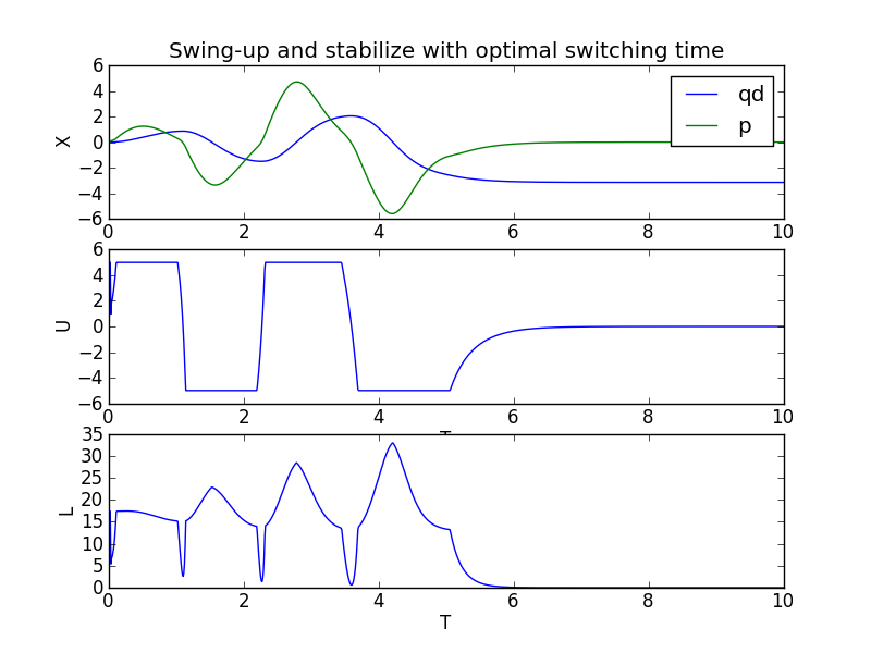
Once the optimal switching time is calculated the system can be simulated forward from its initial configuration. It will reach its desired configuration given the constrained input by switching between the two controllers. In addition, this switch is performed at the optimal time.

(K, T, Q, X, Fdx, E, U, L, J) = simulateForward(tau, dsys, q0, xBar)

From the output of the simulation you can see that it take 3 iteration to converge to the optimal switching time of 4.63.

>>> %run optimalSwitchingTime.py
Optimization iteration: 1
Current switch time: 5.00
New switch time: 4.79
Current cost: 9680.81
Parital of cost to switch time: 1.70
---
Optimization iteration: 2
Current switch time: 4.79
New switch time: 4.63
Current cost: 9214.82
Parital of cost to switch time: 0.62
---
Optimization iteration: 3
Current switch time: 4.63
New switch time: 4.63
Current cost: 9204.84
Parital of cost to switch time: 0.00
---
Optimal switch time: 4.63

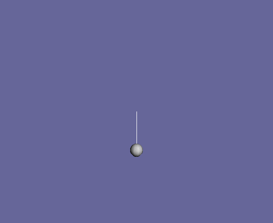
Visualize the system in action

The visualization is created just as in previous sections.

trep.visual.visualize_3d([ trep.visual.VisualItem3D(system, T, Q) ])

# Plot results
ax1 = pylab.subplot(311)
pylab.plot(T, X)
pylab.title("Swing-up and stabilize with optimal switching time")
pylab.ylabel("X")
pylab.legend(["qd","p"])
pylab.subplot(312, sharex=ax1)
pylab.plot(T[1:], U)
pylab.xlabel("T")
pylab.ylabel("U")
pylab.subplot(313, sharex=ax1)
pylab.plot(T[1:], L)
pylab.xlabel("T")
pylab.ylabel("L")
pylab.show()

Let’s also plot the state, input, and cost verse time.

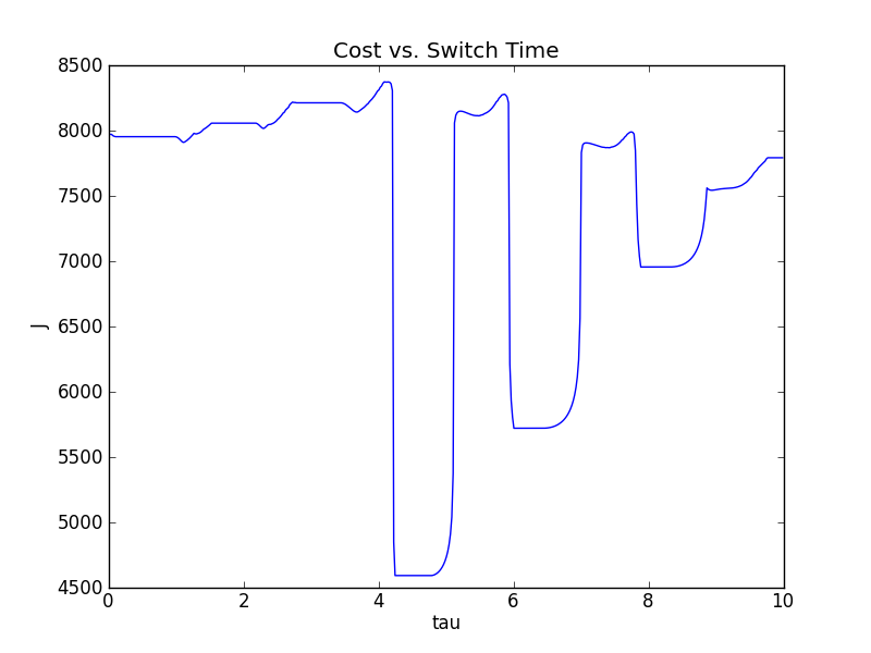
Just for reference the cost verse switching time is shown for all switching times from time zero to the final time. You can see that the optimization does find a switching time with a local minimum in the cost. Clearly, this cost verse switching time is non-convex, thus our gradient descent method only finds a local minimizer, and not a global minimizer.

optimalSwitchingTime.py code

Below is the entire script used in this section of the tutorial.

# optimalSwitchingTime.py

# Import necessary python modules
import math
from math import pi
import numpy as np
from numpy import dot
import trep
import trep.discopt
from trep import tx, ty, tz, rx, ry, rz
import pylab

# Build a pendulum system
m = 1.0 # Mass of pendulum
l = 1.0 # Length of pendulum
q0 = 0. # Initial configuration of pendulum
t0 = 0.0 # Initial time
tf = 10.0 # Final time
dt = 0.01 # Sampling time
qBar = pi # Desired configuration
Qi = np.eye(2) # Cost weights for states
Ri = np.eye(1) # Cost weights for inputs
uMax = 5.0 # Max absolute input value
tau = 5.0 # Switching time

system = trep.System() # Initialize system

frames = [
    rx('theta', name="pendulumShoulder"), [
        tz(-l, name="pendulumArm", mass=m)]]
system.import_frames(frames) # Add frames

# Add forces to the system
trep.potentials.Gravity(system, (0, 0, -9.8)) # Add gravity
trep.forces.Damping(system, 1.0) # Add damping
trep.forces.ConfigForce(system, 'theta', 'theta-torque') # Add input

# Create and initialize the variational integrator
mvi = trep.MidpointVI(system)
mvi.initialize_from_configs(t0, np.array([q0]), t0+dt, np.array([q0]))

# Create discrete system
TVec = np.arange(t0, tf+dt, dt) # Initialize discrete time vector
dsys = trep.discopt.DSystem(mvi, TVec) # Initialize discrete system
xBar = dsys.build_state(qBar) # Create desired state configuration

# Design linear feedback controller
Qd = np.zeros((len(TVec), dsys.system.nQ)) # Initialize desired configuration trajectory
thetaIndex = dsys.system.get_config('theta').index # Find index of theta config variable
for i,t in enumerate(TVec):
    Qd[i, thetaIndex] = qBar # Set desired configuration trajectory
    (Xd, Ud) = dsys.build_trajectory(Qd) # Set desired state and input trajectory

Qk = lambda k: Qi # Create lambda function for state cost weights
Rk = lambda k: Ri # Create lambda function for input cost weights
KVec = dsys.calc_feedback_controller(Xd, Ud, Qk, Rk) # Solve for linear feedback controller gain
KStabilize = KVec[0] # Use only use first value to approximate infinite-horizon optimal controller gain

# Design energy shaping swing-up controller
system.get_config('theta').q = qBar
eBar = system.total_energy()
KEnergy = 1

# Create cost
cost = trep.discopt.DCost(Xd, Ud, Qi, Ri)

# Helper functions
def wrapTo2Pi(ang):
    return ang % (2*pi)

def wrapToPi(ang):
    return (ang + pi) % (2*pi) - pi

def simulateForward(tau, dsys, q0, xBar):
    mvi = dsys.varint
    tf = dsys.time[-1]

    # Reset discrete system state
    dsys.set(np.array([q0, 0.]), np.array([0.]), 0)

    # Initial conditions
    k = dsys.k
    t = dsys.time[k]
    q = mvi.q1
    x = dsys.xk
    fdx = dsys.fdx()
    xTilde = np.array([wrapToPi(x[0] - xBar[0]), x[1]])
    e = system.total_energy() # Get current energy of the system
    eTilde = e - eBar # Get difference between desired energy and current energy

    # Initial list variables
    K = [k] # List to hold discrete update count
    T = [t] # List to hold time values
    Q = [q] # List to hold configuration values
    X = [x] # List to hold state values
    Fdx = [fdx] # List to hold partial to x
    E = [e] # List to hold energy values
    U = [] # List to hold input values
    L = [] # List to hold cost values

    # Simulate the system forward
    while mvi.t1 < tf-dt:
        if mvi.t1 < tau:
            if x[1] == 0:
                u = np.array([uMax]) # Kick if necessary
            else:
                u = np.array([-x[1]*KEnergy*eTilde]) # Swing-up controller
        else:
            u = -dot(KStabilize, xTilde) # Stabilizing controller
        u = min(np.array([uMax]), max(np.array([-uMax]), u)) # Constrain input

        dsys.step(u) # Step the system forward by one time step

        # Update variables
        k = dsys.k
        t = TVec[k]
        q = mvi.q1
        x = dsys.xk
        fdx = dsys.fdx()
        xTilde = np.array([wrapToPi(x[0] - xBar[0]), x[1]])
        e = system.total_energy()
        eTilde = e - eBar
        l = cost.l(np.array([wrapTo2Pi(x[0]), x[1]]), u, k)

        # Append to lists
        K.append(k)
        T.append(t)
        Q.append(q)
        X.append(x)
        Fdx.append(fdx)
        E.append(e)
        U.append(u)
        L.append(l)

    J = np.sum(L)
    return (K, T, Q, X, Fdx, E, U, L, J)

# Optimize
cnt = 0
Tau = []
JVec = []
JdTau = float('Inf')
while cnt < 10 and abs(JdTau) > .001:
    cnt = cnt + 1

    # Simulate forward from 0 to tf
    (K, T, Q, X, Fdx, E, U, L, J) = simulateForward(tau, dsys, q0, xBar)

    # Simulate backward from tf to tau
    k = K[-1]
    lam = np.array([[0],[0]])
    while T[k] > tau + dt/2:
       lamDx = np.array([cost.l_dx(X[k], U[k-1], k)])
       f2Dx = Fdx[k]
       lamDt = -lamDx.T - dot(f2Dx.T,lam)
       lam = lam - lamDt*dt
       k = k - 1

    # Calculate dynamics of swing-up controller at switching time
    x = X[k]
    xTilde = np.array([wrapToPi(x[0] - xBar[0]), x[1]])
    u1 = -dot(KStabilize, xTilde)
    u1 = min(np.array([uMax]), max(np.array([-uMax]), u1))
    dsys.set(X[k], u1, k)
    f1 = dsys.f()

    # Calculate dynamics of stabilizing controller at switching time
    eTilde = E[k] - eBar
    u2 = np.array([-x[1]*KEnergy*eTilde])
    u2 = min(np.array([uMax]), max(np.array([-uMax]), u2))
    dsys.set(X[k], u2, k)
    f2 = dsys.f()

    # Calculate value  of change in cost to change in switch time
    JdTau = dot(f1-f2, lam)

    # Armijo - used to determine step size
    chi = 0
    alpha = .5
    beta = .1
    tauTemp = tau - (alpha**chi)*JdTau
    (KTemp, TTemp, QTemp, XTemp, FdxTemp, ETemp, UTemp, LTemp, JTemp) = simulateForward(tauTemp, dsys, q0, xBar)
    while JTemp > J + (alpha**chi)*beta*(JdTau**2):
        tauTemp = tau - (alpha**chi)*JdTau
        (KTemp, TTemp, QTemp, XTemp, FdxTemp, ETemp, UTemp, LTemp, JTemp) = simulateForward(tauTemp, dsys, q0, xBar)
        chi = chi + 1
    gamma = alpha**chi # Step size

    # Calculate new switching time
    tauPlus = tau - gamma*JdTau

    # Print iteration results
    print "Optimization iteration: %d" % cnt
    print "Current switch time: %.2f" % tau
    print "New switch time: %.2f" % tauPlus
    print "Current cost: %.2f" % J
    print "Parital of cost to switch time: %.2f" % JdTau
    print ""

    # Update to  new switching time
    tau = tauPlus

print "Optimal switch time: %.2f" % tau

# Simulate with optimal switching time
(K, T, Q, X, Fdx, E, U, L, J) = simulateForward(tau, dsys, q0, xBar)

# Visualize the system in action
trep.visual.visualize_3d([ trep.visual.VisualItem3D(system, T, Q) ])

# Plot results
ax1 = pylab.subplot(311)
pylab.plot(T, X)
pylab.title("Swing-up and stabilize with optimal switching time")
pylab.ylabel("X")
pylab.legend(["qd","p"])
pylab.subplot(312, sharex=ax1)
pylab.plot(T[1:], U)
pylab.xlabel("T")
pylab.ylabel("U")
pylab.subplot(313, sharex=ax1)
pylab.plot(T[1:], L)
pylab.xlabel("T")
pylab.ylabel("L")
pylab.show()